Participants and ethics

Participants were recruited from five large hospital sites in London, the United Kingdom: the Great Ormond Street Hospital NHS Foundation Trust, the University College London Hospitals NHS Foundation Trust, the Royal Free London NHS Foundation Trust (the Royal Free Hospital and the Barnet Hospital) and the Whittington Health NHS Trust from March 2020 to February 2021. All participants provided written informed consent. Ethics approval was given through the Living Airway Biobank, administered through the UCL Great Ormond Street Institute of Child Health (REC reference: 19/NW/0171, IRAS project ID: 261511, Northwest Liverpool East Research Ethics Committee). Exclusion criteria for the cohort included current smokers, active haematological malignancies or cancer, known immunodeficiencies, sepsis from any cause and blood transfusions within 4 weeks, known bronchial asthma, diabetes, hay fever and other known chronic respiratory diseases such as cystic fibrosis, interstitial lung disease and chronic obstructive pulmonary disease. Nasal brushings were obtained by trained clinicians from healthy paediatric (0–11 years), adult (30–50 years) and older adult (≥70 years) donors who tested negative for SARS-CoV-2 (within 24–48 h of sampling) and reported no respiratory symptoms in the preceding 7 weeks. Brushings were taken from the inferior nasal concha zone using cytological brushes (Scientific Laboratory Supplies, CYT1050). All methods were performed following the relevant guidelines and regulations. Details of the study population are shown in Supplementary Table 1.

Differentiated human nasal epithelial cell culture

Human nasal brushings were collected fresh for this study and immediately placed in a 15 ml sterile Falcon tube containing 4 ml of transport medium (αMEM supplemented with 1× penicillin/streptomycin (Gibco, 15070), 10 ng ml−1 gentamicin (Gibco, 15710) and 250 ng ml−1 amphotericin B (ThermoFisher, 10746254)) on ice. Four matched paediatric nasal brush samples were sent directly for scRNA-seq9. To minimize sample variation, all samples were processed within 24 h of collection and cultured to P1 as previously described52. Briefly, biopsies were co-cultured with 3T3-J2 fibroblasts and Rho-associated protein kinase inhibitor (Y-27632) in epithelial cell expansion medium consisting of a 3:1 ratio DMEM:F12 (Gibco, 21765), 1× penicillin/streptomycin and 5% FBS (Gibco; 10270) supplemented with 5 μM Y-27632 (Cambridge Bioscience, Y1000), 25 ng ml−1 hydrocortisone (Sigma, H0888), 0.125 ng ml−1 EGF (Sino Biological, 10605), 5 μg ml−1 insulin (Sigma, I6634), 0.1 nM cholera toxin (Sigma, C8052), 250 ng ml−1 amphotericin B (Gibco, 10746254) and 10 μg ml−1 gentamicin (Gibco, 15710).

Basal cells were separated from the co-culture flasks by differential sensitivity to trypsin and seeded onto collagen I-coated, semi-permeable membrane supports (Transwell, 0.4 µm pore size, Corning). Cells were submerged for 24–48 h in an epithelial cell expansion medium, after which the apical medium was removed, and the basolateral medium was exchanged for epithelial cell differentiation medium to generate ‘air–liquid interface’ (ALI) conditions. PneumaCult ALI medium (STEMCELL Technologies, 05001) was used for differentiation media following manufacturer instructions. Basolateral media were exchanged in all cultures three times a week and maintained at 37 °C and 5% CO2. ALI cultures were maintained in PneumaCult ALI medium for 4 weeks to produce differentiated NECs for all downstream experimentation.

Wound healing assay

Mechanical injury of NEC cultures was performed by aspiration in direct contact with the apical cell layer using a P200 sterile pipette tip, creating a wound with a diameter ranging from 750 to 1,500 μm. After wounding, the apical surface of the culture was washed with 200 μl PBS to remove cellular debris. The area of the wound was tracked with the aid of time-lapse microscopy with images taken every 60 min at ×4 magnification (Promon, AIS v.4.6.0.5.). The wound area was calculated each hour using ImageJ. The initial wound area was expressed as 100% to account for variability of wound size. Wounds were considered to be closed when the calculated area fell below 2%, the effective limit of detection due to image processing. Wound closure was calculated as follows: Wound closure (%) = 100 − ((Area/Initial Area) × 100). Wound closure (%) plotted as a function of time (h) was used to calculate the rate of wound closure (% h−1).

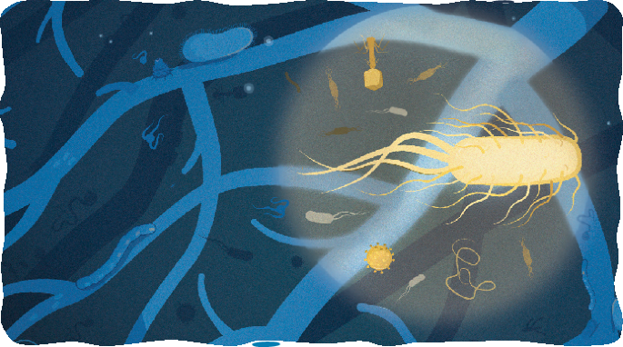
Virus propagation

The SARS-CoV-2 isolate hCoV-19/England/2/2020 obtained from Public Health England (PHE) was used in this study. For virus propagation, the African green monkey kidney cell line Vero E6 (ATCC: CVCL_0574; a kind gift from The Francis Crick Institute, London, United Kingdom and authenticated for use in this study) was used. Vero E6 cells were maintained in DMEM supplemented with 5% FCS and 1× penicillin/streptomycin. Cell media were replenished three times a week and maintained at 37 °C and 5% CO2. Vero E6 cells were infected with an MOI of 0.01 p.f.u. per cell in serum-free DMEM supplemented with 1% NEAA, 0.3% (w/v) BSA and 1× penicillin/streptomycin. A mock condition was conducted in parallel in which an equivalent volume of PBS++ was used instead of viral inoculum. The viral and mock-inoculated cell media were collected after 48 h, centrifuged at 10,000 g for 10 min to remove cellular debris and stored at −70 °C. The viral titre was determined by plaque assay (see below).

Viral infection of NEC cultures

After 28 days, NEC cultures were rinsed with sterile PBS++ and then infected with viral inoculum suspended in PBS++ (4.5 × 104 p.f.u. ml−1, ~0.1 MOI) or an equivalent volume of mock inoculum suspended in PBS++ (mock infection) for 1 h on the apical compartment at 37 °C and 5% CO2. The virus inocula were then removed, and the NEC cultures were washed with sterile PBS++ and incubated for up to 72 h. This timepoint was chosen as maximum viral replication was observed at days 2–3 in our pilot studies (Extended Data Fig. 3a).

Infectious viral load quantification by plaque assay

Vero E6 cells were grown to confluence on 24-well plates and then inoculated with serial dilutions of apical supernatant and cell lysates from infected cultures for 1 h at 37 °C and 5% CO2. The inoculum was replaced by an overlay medium supplemented with 1.2% (w/v) cellulose and incubated for 48 h at 37 °C and 5% CO2. Plates were fixed with 4% (w/v) paraformaldehyde for 30 min and overlay was aspirated from individual wells. Crystal violet staining was performed for a minimum of 20 min, and then plates were washed with water. The number of visible plaques was counted.

Viral copy number quantification

Viral gene quantification was performed on apical wash supernatants from experiments. Samples were lysed in AVL buffer (Qiagen) and stored at −80 °C until further processing. Viral RNA extractions were performed using a QIAamp viral RNA kit (Qiagen) following manufacturer instructions. Extracted RNA samples (5 μl) were quantified in one-step RT–qPCR using AgPath-ID one-step RT–PCR (Applied Biosystems) with the following cycle conditions: 45 °C for 10 min, 95 °C for 15 min, (95 °C for 15 s + 58 °C for 30 s) in a total of 45 cycles.

Cellular gene quantification was performed with cultured cells collected at the end of the experiments. Cells were lysed in RLT buffer (Qiagen) and extraction was performed using an RNeasy mini kit (Qiagen) following manufacturer instructions. Total RNA was converted into cDNA with qScript cDNA supermix (Quantabio) following manufacturer instructions. RT–qPCR was performed using TaqMan Fast Advanced Master mix with the following cycle conditions: 50 °C for 2 min, 95 °C for 10 min, 95 °C for 30 s and 60 °C for 1 min in a total of 45 cycles. The expression was normalized with GAPDH and then presented as 2−(ΔCт) in arbitrary units.

SARS-CoV-2 genomic sequencingViral genome read coverage

To visualize the viral read coverage along the viral genome, we used the 10X Genomics cellranger barcoded binary alignment map (BAM) files for every sample. We filtered the BAM files to only retain reads mapping to the viral genome using the bedtools intersect tool52. We converted the BAM files into sequence alignment map (SAM) files to filter out cells that were removed in our single-cell data pre-processing pipeline. The sequencing depth for each base position was calculated using samtools count. To characterize read distribution along the viral genome, we counted transcripts of 10 different open reading frames (ORFs): ORF1ab, Surface glycoprotein (S), ORF3a, Envelope protein (O), Membrane glycoprotein (M), ORF6, ORF7a, ORF8, Nucleocapsid phosphoprotein (N) and ORF10.

Detection of SARS-CoV-2 subgenomic RNAs

Subgenomic RNA analysis was conducted using Periscope53. Briefly, Periscope distinguished sgRNA reads on the basis of the 5′ leader sequences being directly upstream from each gene’s transcription. The sgRNA counts were then normalized into a measure termed sgRPTL, by dividing the sgRNA reads by the mean depth of the gene of interest and multiplying by 1,000.

ProteomicsMass spectrometry

Paired mock- and SARS-CoV-2-infected airway surface fluids from groups of 10 paediatric, adult and older adult cultures were selected for this assay. For mass spectrometry, samples were inactivated with the KeyPro UV LED decontamination system (Phoseon Technology) before removal from the Biosafety level 3 laboratory (BSL3). Proteins were precipitated using ice-cold acetone. Protein pellets were resuspended in the digestion buffer as previously described and trypsin (Promega) digested to peptides54. Peptides were desalted by solid phase extraction (SPE) and separated by reverse phase chromatography on a NanoAquity LC system coupled to a SYNAPT G2-Si mass spectrometer (Waters) in a UDMSE positive ion electrospray ionization mode. Raw MS data were processed using Progenesis QI analysis software (Nonlinear Dynamics). Peptide identification was performed using the UniProt human reference proteome, with one missed cleavage and 1% peptide false discovery rate (FDR). Fixed modifications were set to carbamidomethylation of cysteines and dynamic modifications of oxidation of methionine.

Western blot

Samples were resolved on 4–15% Mini-PROTEAN TGX Precast Protein Gel (Bio-rad, 4561083) with high molecular mass standards of 10–250 kDa. Proteins were transferred to a Trans-Blot Turbo Mini 0.2 µm nitrocellulose membrane in a Trans-Blot Turbo Transfer System (Bio-rad, 1704150). Membranes were blocked in Odyssey blocking buffer overnight at 4 °C. Membranes were probed with primary antibodies described in Supplementary Table 2, with dilutions prepared in Odyssey blocking buffer. Incubation with primary antibodies was performed at room temperature (r.t.) for 1 h. These included rabbit anti-ACE2 recognizing both long and short isoforms (Abcam, ab15348, 1:2,000) and rabbit anti-ACE2 specific for the long isoform (Abcam, ab108252, 1:2,000), rat anti-alpha-tubulin (Sigma-Aldrich, MAB1864, 1:2,000) and acetylated forms (Sigma-Aldrich, T6793, 1:2,000), mouse anti-SARS-CoV-2 spike glycoprotein (Abcam, ab273433, 1:2,000), rabbit anti-GAPDH (Abcam, ab9485, 1:3,000), rabbit anti-vimentin (Abcam, ab16700, 1:500) and rabbit anti-E-cadherin (Abcam, ab40772, 1:10,000). After three 15 min washes in PBS containing 0.1% Tween 20, the membranes were incubated with the appropriate IRDye secondary antibodies: goat anti-mouse (LI-COR, 926-68070, dilution 1:18,000) and goat anti-rabbit (LI-COR, 926-32211, dilution 1:18,000), both at room temperature for 1 h. The blots were then visualized using an Odyssey CLx imager and quantified using Image Studio Lite software

Cytokine assay

Apical supernatants were collected by washing the apical surface with 200 μl of PBS. These were snap frozen at −70 °C and inactivated with the KeyPro UV LED decontamination system (Phoseon Technology) in the CL3 laboratory before handling them in a CL2 laboratory. Cytokine and chemokine levels were assessed in 25 μl of supernatants using the multiplex BD CBA bead-based immunoassay kits including: IL6: A7, 558276; IL8 (CXCL8): A9, 558277; TNFα: C4, 560112; IFNγ: E7, 558269; IP10 (CXCL10): B5, 558280; IFNα: B8, 560379; and IL10: B7, 558274. Data were acquired using the BD LSRII flow cytometer and concentrations were obtained from a standard curve (provided with the kit). Analysis was performed using the FCAP software (v.3.0, BD Biosciences).

MicroscopyImmunofluorescence confocal microscopy

For immunofluorescence confocal imaging, NEC cultures were fixed using 4% (v/v) paraformaldehyde for 30 min, permeabilized with 0.2% Triton X-100 (Sigma) for 15 min and blocked using 5% goat serum (Sigma) in PBS for 1 h. The cultures were then incubated overnight at 4 °C with primary antibodies described in Supplementary Table 2, with dilutions prepared in 5% goat serum in PBS with 0.1% Triton X-100. The primary antibodies used included rabbit anti-ACE2 (Abcam, ab15348, diluted 1:200), mouse anti-MUC5AC (Sigma-Aldrich, MAB2011, diluted 1:500), rat anti-alpha-tubulin (tyrosinated) (Sigma-Aldrich, MAB1864, diluted 1:100), mouse anti-alpha-tubulin (acetylated) (Sigma-Aldrich, T6793, diluted 1:100), mouse anti-SARS-CoV-2 spike glycoprotein (Abcam, ab273433, diluted 1:500), rabbit anti-GAPDH (Abcam, ab9485, diluted 1:250), mouse anti-dsRNA (Jena Bioscience, RNT-SCI-10010500, diluted 1:100), rabbit anti-MX1 (Abcam, ab207414, diluted 1:250), rabbit anti-cytokeratin 5 conjugated with Alexa Fluor 647 (Abcam, ab193895, diluted 1:100), rabbit anti-vimentin (Abcam, ab16700, diluted 1:1,000), rabbit anti-IL28+29 (Abcam, ab191426, diluted 1:100), goat anti-BPIFA1 (Abcam, EB11482, diluted 1:100) and rat anti-integrin beta 6 (Abcam, ab97588, diluted 1:100).

Following primary antibody incubation, cultures were washed and then incubated with secondary antibodies diluted in 1.25% goat serum in PBS with 0.1% Triton X-100 at r.t. for 1 h the following day. The secondary antibodies included donkey anti-mouse Alexa Fluor 647 (Jackson ImmunoResearch, 715-605-151, 1:600), donkey anti-rat Alexa Fluor 647 (Jackson ImmunoResearch, 712-605-153, 1:600), donkey anti-mouse Alexa Fluor 594 (Jackson ImmunoResearch, 715-585-151, 1:600), donkey anti-rat Alexa Fluor 594 (Jackson ImmunoResearch, 712-585-153, 1:600), donkey anti-mouse Cy3 (Jackson ImmunoResearch, 715-165-151, 1:600), donkey anti-rabbit Cy3 (Jackson ImmunoResearch, 711-165-152, 1:600), donkey anti-rat Alexa Fluor 488 (Jackson ImmunoResearch, 712-545-153, 1:600), donkey anti-rabbit Alexa Fluor 488 (Jackson ImmunoResearch, 711-545-152, 1:600), donkey anti-mouse Alexa Fluor 488 (Jackson ImmunoResearch, 715-545-151, 1:600) and donkey anti-goat Alexa Fluor 488 (Jackson ImmunoResearch, 705-545-147, 1:600).

After the secondary antibody incubation, cultures were stained with Alexa Fluor 555 phalloidin (ThermoFisher, A34055, 4 μg ml−1) for 1 h and DAPI (Sigma, 2 μg ml−1) for 15 min at r.t. to visualize F-actin and nuclei, respectively. Samples were washed three times with PBS containing 0.1% Tween 20 after each incubation step.

Imaging was carried out using an LSM710 Zeiss confocal microscope, and the resulting images were analysed using Fiji/ImageJ v.2.1.0/153c54 for metrics including mean intensity, cell protrusion, culture thickness, % signal coverage, wound area and pseudocolouring55. Intensity profiles were generated using Nikon NIS-Elements analysis module, and three-dimensional (3D) renderings of immunofluorescence images were produced with Imaris software (Bitplane, Oxford Instruments; v.9.5/9.6).

Transmission electron microscopy

Cultured NECs that were either SARS-CoV-2-infected or non-infected were fixed with 4% paraformaldehyde and 2.5% glutaraldehyde in 0.05 M sodium cacodylate buffer at pH 7.4 and placed at 4 °C for at least 24 h. The samples were incubated in 1% aqueous osmium tetroxide for 1 h at r.t. before subsequent en bloc staining in undiluted UA-Zero (Agar Scientific) for 30 min at r.t. The samples were dehydrated using increasing concentrations of ethanol (50, 70, 90, 100%), followed by propylene oxide and a mixture of propylene oxide and araldite resin (1:1). The samples were embedded in araldite and left at 60 °C for 48 h. Ultrathin sections were acquired using a Reichert Ultracut E ultramicrotome and stained using Reynold’s lead citrate for 10 min at r.t. Images were taken on a JEOL 1400Plus TEM equipped with an Advanced Microscopy Technologies (AMT) XR16 charge-coupled device (CCD) camera and using the AMT Capture Engine software.

Sample preparation for single-cell RNA sequencing

Cultured NECs were processed using an adapted cold-active protease single-cell dissociation protocol56, as described below, based on a previously used protocol9 to allow for a better comparison of matched samples included in both studies. In total, NECs derived from n = 3 paediatric, 4 adult and 4 older adult donors were processed at 24, 48 and 72 h post infection (SARS-CoV-2 and mock) for scRNA-seq.

First, the transwell inserts, in which the NEC cultures were grown, were carefully transferred into a new 50 ml Falcon tube and any residual transport medium was carefully removed so as not to disturb the cell layer. Dissociation buffer (2 ml) was then added to each well, ensuring the cells were covered; 10 mg ml−1 protease from Bacillus licheniformis (Sigma-Aldrich, P5380) and 0.5 mM EDTA in HypoThermosol (STEMCELL Technologies, 07935). The cells were incubated on ice for 1 h. Every 5 min, cells were gently triturated using a sterile blunt needle, decreasing from a 21G to a 23G needle. Following dissociation, protease was inactivated by adding 400 µl of inactivation buffer (HBSS containing 2% BSA) and the cell suspension was transferred to a new 15 ml Falcon tube. The suspension was centrifuged at 400 g for 5 min at 4 °C and the supernatant was discarded. Cells were resuspended in 1 ml dithiothreitol wash (10 mM dithiothreitol in PBS) (ThermoFisher, R0861) and gently mixed until any remaining visible mucous appears to break down, or for ~2–4 min. The mixture was centrifuged at 400 g for 5 min at 4 °C and the supernatant was removed. The cells were resuspended in 1 ml of wash buffer (HBSS containing 1% BSA) and centrifuged once more under the same conditions. The single-cell suspension was then filtered through a 40 µm Flowmi cell strainer. Finally, the cells were centrifuged and resuspended in 30 µl of resuspension buffer (HBSS containing 0.05% BSA). Using trypan blue, total cell counts and viability were assessed. Cells (3,125) were then pooled together from the 4 biological replicates with corresponding conditions (for example, all mock viral treatments at 24 h) and the cell concentration was adjusted for 7,000 targeted cell recovery according to the 10x Chromium manual (between 700–1,000 cells per µl). The pools were then processed immediately for 10 × 5′ single-cell capture using the Chromium Next GEM Single Cell V(D)J reagent kit v.1.1 (Rev E Guide) or the Chromium Next GEM Single Cell 5′ V2 (Dual index) kit (Rev A guide). Each pool was run twice.

Of note, each sample was processed fresh for 5’ Next Gen single-cell RNA sequencing and thus pooled per timepoint when loading on the 10X chromium controller. Extra steps were taken where possible to balance sex, age as well as technical factors (that is, 10X chromium kit versions) within these sample pools. Furthermore, the downstream process of the sample pools, including library preparation and sequencing (see below) contained samples from the 4 h, 24 h and 72 h timepoints to mitigate additional technical effects. Timepoints can be seen to be well mixed within the single-cell dataset as visualized via a uniform manifold approximation and projection (UMAP) in Extended Data Fig. 1b.

For several samples (Supplementary Table 3), 1 µl viral RT oligo (either at 5 µM or 100 µM, PAGE) was spiked into the master mix (at step 1.2.b in the 10X guide, giving a final volume of 75 µl) to help with the detection of SARS-CoV-2 viral reads. The samples were then processed according to manufacturer instructions, with the viral cDNA separated from the gene expression libraries (GEX) by size selection during step 3.2. Here the supernatant was collected (159 µl) and transferred to a new PCR tube and incubated with 70 µl of SPRI beads (0.6× selection) at r.t. for 5 min. The SPRI beads were then washed according to the guide and the viral cDNA was eluted using 30 µl of EB buffer. Neither changes to the transcriptome were previously observed upon testing the addition of viral oligo9, nor were any significant changes observed with an increasing concentration upon comparison, outside of a small increase in the overall number of SARS-CoV-2 reads detected. The RT oligo sequence was as follows: 5′-AAGCAGTGGTATCAACGCAGAGTACTTACTCGTGTCCTGTCAACG-3′

Library generation and sequencing

The Chromium Next GEM Single Cell 5′ V2 kit (v.2.0 chemistry) was used for single-cell RNA-seq library construction. For all NEC culture samples, libraries were prepared according to manufacturer protocol (10X Genomics) using individual Chromium i7 sample indices. GEX libraries were pooled and sequenced on a NovaSeq 6000 S4 flow cell (paired-end, 150 bp reads), aiming for a minimum of 50,000 paired-end reads per cell for GEX libraries.

Single-cell RNA-seq data processingComputational pipelines, processing and analysis

The single-cell data were mapped to a GRCh38 ENSEMBL 93 derived reference, concatenated with 21 viral genomes (featuring SARS-CoV-2), of which the NCBI reference sequence IDs are: NC_007605.1 (EBV1), NC_009334.1 (EBV2), AF156963 (ERVWE1), AY101582 (ERVWE1), AY101583 (ERVWE1), AY101584 (ERVWE1), AY101585 (ERVWE1), AF072498 (HERV-W), AF127228 (HERV-W), AF127229 (HERV-W), AF331500 (HERV-W), NC_001664.4 (HHV-6A), NC_000898.1 (HHV-6B), NC_001806.2 (herpes simplex virus 1), NC_001798.2 (herpes simplex virus 2), NC_001498.1 (measles morbillivirus), NC_002200.1 (mumps rubulavirus), NC_001545.2 (rubella), NC_001348.1 (varicella zoster virus), NC_006273.2 (cytomegalovirus) and NC_045512.2 (SARS-CoV-2). When examining viral load per cell type, we first removed ambient RNA by SoupX57. The alignment, quantification and preliminary cell calling of NEC culture samples were performed using the STARsolo functionality of STAR v.2.7.3a, with the cell calling subsequently refined using the Cell Ranger v.3.0.2 version of EmptyDrops58. Initial doublets were called on a per-sample basis by computing Scrublet scores59 for each cell, propagating them through an over-clustered manifold by replacing individual scores with per-cluster medians and identifying statistically significant values from the resulting distribution, replicating previous approaches60,61.

Quality control, normalization and clustering

Mixed genotype samples were demultiplexed using Souporcell62 and reference genotypes. DNA from samples was extracted following manufacturer protocol (Qiagen, DNeasy blood and tissue kit 69504 and Qiagen Genomic DNA miniprep kit) and single nucleotide polymorphism (SNP) array-derived genotypes generated by Affymetrix UK Biobank Axiom Array kit by Cambridge Genomic Services (CGS). Cells that were identified as heterotypic doublets by Souporcell were discarded. Quality control was performed on SoupX-cleaned expression matrixes. Genes with fewer than 3 counts and cells with more than 30% mitochondrial reads were filtered out. Cells with a scrublet score >0.3 and adjusted P value < 0.8 were predicted as doublets and filtered out. Expression values were then normalized to a sum of 1 × 104 per cell and log-transformed with an added pseudocount of 1. Highly variable genes were selected using the scanpy.pp.highly_variable_genes() function in Scanpy. Principal component analysis (PCA) was performed and the top 30 principal components were selected as input for l. We performed graph-based batch integration with the bbknn method63 using experimental pools and chemistry as batch covariate (encoded as ‘bbknn_batch’ in the object). Clustering was performed with the Leiden64 algorithm on a k-nearest-neighbour graph of a PCA space derived from a log(counts per million/100 + 1) representation of highly variable genes, according to the Scanpy protocol65. Leiden clustering with a resolution of 1 was used to separate broad cell types (basal, goblet, secretory). For each broad cell type, clustering was then repeated, starting from highly variable gene discovery to achieve a higher resolution and a more accurate separation of refined cell types. Annotation was first performed automatically using a Celltypist66 model built on the in vivo dataset of nasal airway brushes9, and then using manual inspection of each of the clusters and further manual annotation using known airway epithelial marker genes.

Developmental trajectory inference

Pseudotime inference was performed on the whole object or the basal/goblet compartment using Monocle 3 (refs. 67,68). Briefly, a cycling basal cell was chosen as a ‘root’ cell for the basal compartment, showing the highest combined expression of KRT5, MKI67 and NUSAP1 genes. For the goblet compartment, a goblet 1 cell was chosen as a root, showing the highest combined expression of TFF3, SERPINB3, MUC5AC, MUC5B and AQP5. Cells were grouped into different clusters using the group_cells() function, learning the principal graph using the learnGraph() function and ordering cells along the trajectory using the ordercells() function. A second pseudotime was inferred with Palantir (1.0.1)69. The cycling basal ‘root’ cell was determined as above and an unsupervised pseudotime inference was performed on a Scanpy-derived diffusion map. The five inferred endpoints were inspected and three were deemed to be very closely biologically related and replaced with a joint endpoint with the highest combined expression of OMG, PIFO and FOXJ1. The pseudotime inference was repeated with the two remaining inferred endpoints and the marker derived one serving as the three terminal states.

Differential abundance analysis

To determine cell states that are enriched in the SARS-CoV-2 versus mock conditions for the different age groups, we used the Milo framework for differential abundance analysis using cell neighbourhoods14. Briefly, we computed k-nearest-neighbour graphs of cells in the whole dataset using the buildGraph() function, assigned cells to neighbourhoods using the makeNhoods() function and counted the number of cells belonging to each sample using the countCells() function. Each neighbourhood was assigned the original cluster labels using majority voting. To test for enrichment of cells in the SARS-CoV-2 condition versus the mock condition, we modelled the cell count in neighbourhoods as a negative binomial generalized linear model, using a log-linear model to model the effects of age and treatment on cell counts (logFC). We control for multiple testing using the weighted Benjamini–Hochberg correction as described in ref. 14 (spatialFDR correction). Neighbourhoods were considered enriched in SARS-CoV-2 vs mock if the spatialFDR < 0.1 and logFC > 0.

Expression signature analysis

To determine the enrichment of basaloid or interferon genes in the annotated clusters, we used the Scanpy function scanpy.tl.score_genes() to score the gene signature for each cell. The gene list for computing the basaloid score was composed of the EPCAM, CDH1, VIM, FN1, COL1A1, CDH2, TNC, VCAN, PCP4, CUX2, SPINK1, PRSS2, CPA6, CTSE, MMP7, MDK, GDF15, PTGS2, SLCO2A1, EPHB2, ITGB8, ITGAV, ITGB6, TGFB1, KCNN4, KCNQ5, KCNS3, CDKN1A, CDKN2A, CDKN2B, CCND1, CCND2, MDM2, HMGA2, PTCHD4 and OCIAD2 genes. The gene list for computing the IFN alpha score was composed of the ADAR, AXL, BST2, EIF2AK2, GAS6, GATA3, IFIT2, IFIT3, IFITM1, IFITM2, IFITM3, IFNAR1, IFNAR2, KLHL20, LAMP3, MX2, PDE12, PYHIN1, RO60, STAR and TPR genes and the gene list for computing the IFN gamma score was composed of the OAS3, OASL, OTOP1, PARP14, PARP9, PDE12, PIAS1, PML, PPARG, PRKCD, PTAFR, PTPN2, RAB20, RAB43, RAB7B, RPL13A, RPS6KB1, SHFL, SIRPA, SLC11A1, SLC26A6, SLC30A8, SNCA, SOCS1, SOCS3, SP100, STAR, STAT1, STX4, STX8, STXBP1, STXBP3, STXBP4, SUMO1, SYNCRIP, TDGF1, TLR2, TLR3, TLR4, TP53, TRIM21, TRIM22, TRIM25, TRIM26, TRIM31, TRIM34, TRIM38, TRIM5, TRIM62, TRIM68, TRIM8, TXK, UBD, VAMP3, VCAM1, VIM, VPS26B, WAS, WNT5A, XCL1, XCL2, ZYX genes, as used in ref. 9.

Gene set enrichment analysis

Wilcoxon rank-sum test was performed to determine differentially expressed genes between clusters using the scanpy.tl.rank_genes_groups() function. Differentially expressed genes were further analysed using GSEA via ShinyGO70.

In vivo sub-analysis

Sex- and age-matched healthy adults and paediatric airway samples (n = 10 total) were subsetted from our previous dataset9 for label transfer of the in vitro cell annotation using CellTypist as described above. Selected sample IDs from the in vivo dataset are shown in Supplementary Table 4. These were selected to match the mean age and range, and sex of the current study as the sample collection and processing were conducted in parallel between studies.

In vivo integration

We performed integration of 8 single-cell datasets comprising 614,695 cells from upper and lower airways from healthy and COVID-19 patients from paediatric (0–18 years), adult (19–50 years) and older adult (51–90 years) samples9,10,12,18,19,20,21,22. Expression values were then normalized to a sum of 1 × 104 per cell and log-transformed with an added pseudocount of 1. Highly variable genes were selected using the Scanpy function scanpy.pp.highly_variable_genes(). PCA was performed and the top 30 principal components were selected as input for Harmony71 to correct for batch effects between studies and compute a batch-corrected k-nearest-neighbour graph. The clustering was performed with the Leiden64 algorithm on a k-nearest-neighbour graph of a PCA space derived from a log(counts per million/100 + 1) representation of highly variable genes, according to the Scanpy protocol65. Leiden clustering with a resolution of 1 was used to separate broad cell types (basal, goblet, secretory) and subclustering was used for more accurate separation of fine-grained cell types. Annotation was first performed automatically using a Celltypist66 model built on the in vivo dataset of nasal airway brushes9, and then using manual inspection of each of the clusters and further manual annotation using known epithelial marker genes.

Statistical analysis on in vivo dataset

Due to the large proportions of zero counts, we fitted zero-inflated Poisson (ZIP) models to the counts of nasal epithelial cells including the natural logarithm of the total number of cells per donor as an offset in the models for both basaloid and gobletInFam cells. This allowed us to estimate both the incidence of nasal epithelial cells () and the probability of a donor being in the zero counts class () as functions of disease and age groups. We first included interaction terms between the disease and age groups in both the incidence and the zero counts parts of the models. Generalized additive models for location, scale and shape were fitted using the packages gamlss72 and glmmTMB73 (to include random effects on the probability of zero class by donor), both in the R language and environment for statistical computing (v.4.2.3)74. Using the Bayesian Information Criterion (BIC) as a goodness-of-fit statistic, we decided to include the main effects of disease in both the linear predictors for incidence and probability of belonging to the zero class after stratifying by age group.

Statistical analysis

Statistical analysis was performed using R or GraphPad Prism 9 and details of statistical tests used are indicated. Data distribution was assumed to be normal unless stated differently, and a Kruskal–Wallis test was used to test for normality using R. The determination of sample sizes was guided by those established in previous scRNA-seq and studies using ALI cultures9,75, rather than through the application of specific statistical methods. In total, NEC cultures generated from 11 participants were used to create our in vitro single-cell dataset, including 3 paediatric (<12 years), 4 adult (30–50 years) and 4 older adult (>70 years) donors. Additional statistical power here was provided by the experimental design, sampling from multiple timepoints (4, 24 and 72 h post SARS-CoV-2 infection), with the inclusion of matched mock-infected controls for each. Samples were also carefully pooled (see Methods) to help avoid batch effects and run across multiple lanes on the 10X controller. Together, this resulted in a total of 66 NEC samples processed for single-cell sequencing, with a total of 139,598 high-quality cells sequenced. Further validation of our in vitro single-cell data and our key observation was provided using an integrated in vivo single-cell dataset (using published patient datasets) and numerous experimental validation assays. Data collection and analysis were not performed blind to the conditions of the experiments. Representative images are displayed as examples for quantified data (1n of the total n noted in their corresponding summary graphs) unless otherwise stated in the figure legend.

Reporting summary

Further information on research design is available in the Nature Portfolio Reporting Summary linked to this article.