1 Introduction

Decoding of cognitive states from the brain activity, or simply the “brain decoding” has emerged as one of the most active research areas because of its potentially wide-ranging implications in medical and therapeutic engineering fields (Santhanam et al., 2006; Hou et al., 2022). Due to its noninvasive approach and considerable spatial and temporal resolution, functional magnetic resonance imaging (fMRI) is commonly used to decode cognitive states. Traditional fMRI techniques use generalized linear models to predict regional brain activity based on specific behavioral tasks or cognitive states that a participant performs or experiences. This approach can mistakenly be interpreted in reverse–assuming specific activation patterns indicate definite cognitive states (Poldrack, 2011; Zhang et al., 2021). However, this is often inaccurate, as patterns of activity by different tasks and states can be overlapping. It's been suggested that reverse inference can be more reliably applied through brain decoding methods, where spatiotemporal activity is used to predict cognitive states under various conditions (Poldrack, 2006; Zhang et al., 2021). Across the wide literature, the terms “cognitive states,” “brain states,” and “task-states” have been used more or less synonymously. To avoid any confusion, we mostly stick with the term “cognitive states,” with few instances of “brain states.” By both, we mean the state of the brain during specific cognitive processes or behavioral tasks.

Although there have been significant improvements in brain decoding about specific cognitive states, there exist also genuine knowledge gap.Previous studies (Haxby et al., 2001; Li and Fan, 2019; Wang et al., 2020) attempted to generate models that could decode brain states across a wide range of behavioral domains. Meta-analytic methodologies have been utilized for multi-domain decoding (Bartley et al., 2018). However, meta-analyses face several limitations, such as inconsistent samples across cognitive domains, publication bias favoring positive results, and inflated effect sizes from small studies (Dubben and Beck-Bornholdt, 2005; Alamolhoda et al., 2017; Lin, 2018; Zhang et al., 2021). In areas with limited research, these issues can bias decoding analyses and lead to incorrect inferences (Lieberman and Eisenberger, 2015; Lieberman et al., 2016; Wager et al., 2016). An alternate method is to overcome these biases by training linear classifiers on activation maps acquired from a group of individuals (Poldrack et al., 2009; Bzdok et al., 2016; Varoquaux et al., 2018; Zhang et al., 2021).

A few studies have employed Deep Neural Network (DNN) models, such as Convolutional Neural Networks (CNNs), which are efficient, scalable, and can differentiate patterns without requiring manual features. 3d CNN-based models are shown to be efficient at decoding states of the brain across multiple domains of stimulus processing (Wang et al., 2020). However, there are some limitations of DNNs; training DNN architectures with fully connected layers is challenging, particularly in neuroimaging applications, because of many free parameters and a limited number of labeled training data. As a result, these architectures tend to overfit the data and exhibit poor out-of-sample prediction (Zhang et al., 2021). Secondly, though DNN performs admirably with grid-like inputs in Euclidean space, such as (natural) images, the distance in Euclidean space may not adequately represent the functional distance between different parts of the brain (see similar; Rosenbaum et al., 2017). Instead, geometric deep-learning (DL) methods, such as graph convolutional networks (GCNs), would better suit non-Euclidean data types, such as brain networks (Zhang and Bellec, 2019; Zhang et al., 2021).

Critically, extant DL approaches do not exploit the dynamic spatiotemporal characteristics of brain activity during naturalistic movie-watching paradigms. These paradigms provide a promising pathway to examine brain dynamics across a diverse spectrum of realistic human experience(s) and provide a rich context-dependent array of cognitive states and sub-states to be investigated with the help of machine learning (ML) models (Simony and Chang, 2020). Also, DNN models that decode brain data from the developmental period are lacking. We believe that modeling stimulus-evoked activity patterns of children and adolescents from naturalistic movie-watching paradigms can more effectively characterize states across multiple cognitive domains, especially, those of higher-order cognition like Theory of Mind (ToM).

To address these challenges, we developed a novel spatiotemporal graph convolutional neural network model (stGCNN) that inputs functional connectivity (FC) and inter-subject functional connectivity (ISFC), derived from BOLD time-series data from key brain regions. This model effectively captures the spatiotemporal dynamics of brain activity to differentiate between brain activation patterns associated with two cognitive states: the perception of others' pain and Theory of Mind (ToM) processing in children and adolescents. Our study aimed to a) develop an explainable spatiotemporal decoding model to classify brain activation patterns using connectivity features, FC and ISFC, during movie watching in children, adolescents, and adults (control), and b) use contributing features from the previous model to predict individual performance on false-belief tasks.

The stGCNN model is based on a graph Laplacian-based model that models the brain as a graph treating region-of-interest (ROI) as nodes and their connectivity as edges. The proposed explainable spatiotemporal connectivity-based graph convolutional neural network (Ex-stGCNN) model accurately decodes time courses during which participants experienced a particular cognitive state while watching the movie (Refer to Figure 1). The proposed model could extract features from non-Euclidean data and process graph-structured signals. We used FC, which reflects inter-regional correlations arising from a mixture of stimulus-induced neural processes, intrinsic neural processes, and non-neuronal noise, and ISFC, which isolates stimulus-dependent inter-regional correlations by modeling the BOLD signal of one brain on the other brain's exposed to the same stimulus (Simony et al., 2016), as feature set to train the proposed model. As a result, we achieved an average of 94 % accuracy with an F1-Score of 0.95. We applied the SHAP (SHapley Additive exPlanations) method for explainability and finally identified neurobiological brain features that contributed the most to the prediction. Then we implemented the unsupervised Explainable Convolutional Variational Autoencoder model (Ex-Convolutional VAE) to predict individual performance in false-belief tasks in which FC and ISFC matrices were used as feature sets. We obtained 90 % accuracy using FC matrices as a feature set with an F1-Score of 0.92% and 93.5% accuracy with an F1-score of 0.94 using ISFC matrices. To validate the results, we implemented Five-fold cross-validation. We have made a comparison with previously employed models and found that our Convolutional Variational Auto Encoder (CVAE) model gave the best prediction accuracy. The final challenge we address here is one of the most interesting questions in neuroscience related to identifying neurobiologically meaningful features at the individual participant level that predict their performance in the cognitive task. To our knowledge, no previous DL classification study in mentalization tasks has investigated neurobiologically interpretable spatiotemporal brain features that robustly predict Theory of Mind task performance in children, adolescents along with adults, without feature engineering. This framework not only decoded brain states for groups of different developmental ages and adults and highly imbalanced datasets with high accuracy from short-time course data but also predicted individual performance in false-belief tasks to classify participants into pass, fail, and inconsistent groups independent of their behavioral performance ratings. Based on our theoretical model, we predict that social cognition networks [comprised of bilateral Temporoparietal Junction (LTPJ and RTPJ), Posterior Cingulate Cortex (PCC), Ventral and Dorsal-medial Prefrontal Cortex (vmPFC and dmPFC), and Precuneus] feature prominently in the prediction of cognitive performance in children and adolescents during early development.

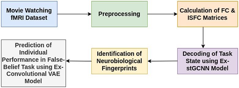
Figure 1. Illustrative overview of end-to-end explainable deep-learning framework for decoding of cognitive states and prediction on performance of false-belief task-based pass, fail, and inconsistent groups.

2 Materials and methods 2.1 Participants and fMRI preprocessing

To develop models for investigating Theory-of-Mind and Pain networks across developmental stages, we analyzed a dataset of 155 early childhood to adult participants, available on the OpenfMRI database. (The childhood group consisted of 122 participants aged 3–12-yrs (mean age = 6.7 yrs, SD = 2.3, 64 females), complemented by 33 adults (mean age = 24.8 yrs, SD = 5.3, 20 females) (Astington and Edward, 2010; Richardson et al., 2018; Bhavna et al., 2023). Participants who participated in the study were from the surrounding neighborhood and brought in a signed permission form from a parent or guardian. The approval for data collection was given by the Committee on the Use of Humans as Experimental Subjects (COUHES) at the Massachusetts Institute of Technology. In this experiment, participants watched a soundless short animated movie of 5.6 min named “Partly Cloudy” (Refer to Figure 2). Using a dataset that included developmental age groups (3–12 yrs) and individuals in adulthood opened the opportunity to propose a framework for the decoding of cognitive states that could analyze complex brain dynamics in the early childhood stage and contextualize these findings from the perspective of adult brains. After scanning, six explicit ToM-related questions were administered for the false-belief task to identify the correlation between brain development and behavioral scores in ToM reasoning. Each child's performance on the ToM-related false-belief task was assessed based on the proportion of questions answered correctly out of 24 matched items (14 prediction items and 10 explanation items). Based on the outcome of these explicit false-belief task scores, the participants were categorized into three classes: Pass (5–6 correct answers), inconsistent (3–4 correct answers), and fail (0–2 correct answers) (Reher and Sohn, 2009; Astington and Edward, 2010; Jacoby et al., 2016; Richardson et al., 2018). A 3-Tesla Siemens Tim Trio scanner at the Athinoula A. Martinos Imaging Center at MIT was used to collect whole-brain structural and functional MRI data (For head coil details, see Richardson et al., 2018). Children under 5 used one of the two custom 32-channel head coils: younger (n = 3, M(s.d.) = 3.91(0.42) yrs) or older (n = 28, M(s.d.) = 4.07(0.42) yrs) children; all other participants used the standard Siemens 32-channel head coil. With a factor of three for GRAPPA parallel imaging, 176 interleaved sagittal slices of 1 mm isotropic voxels were used to get T1-weighted structural images (FOV: 192 mm for child coils, 256 mm for adult coils). The whole brain was covered by 32 interleaved near-axial slices that were aligned with the anterior/posterior commissure and used a gradient-echo EPI sequence sensitive to BOLD contrast to capture functional data (EPI factor: 64; TR: 2 s, TE: 30 ms, flip angle: 90) (Richardson et al., 2018). All functional data were upsampled in normalized space to 2 mm isotropic voxels. Based on the participant's head motion, one TR back, prospective acquisition correction was used to modify the gradient locations. The dataset was preprocessed using SPM 8 and other toolboxes available for Matlab (Penny et al., 2011), which registered all functional images to the first run image and then registered that image to each participant's structural images (Astington and Edward, 2010). All structural images were normalized to Montreal Neurological Institute (MNI) template (Burgund et al., 2002; Cantlon et al., 2006). The smoothing for all images was performed using a Gaussian filter and identified Artifactual timepoints using ART toolbox (Astington and Edward, 2010; Whitfield-Gabrieli et al., 2011).

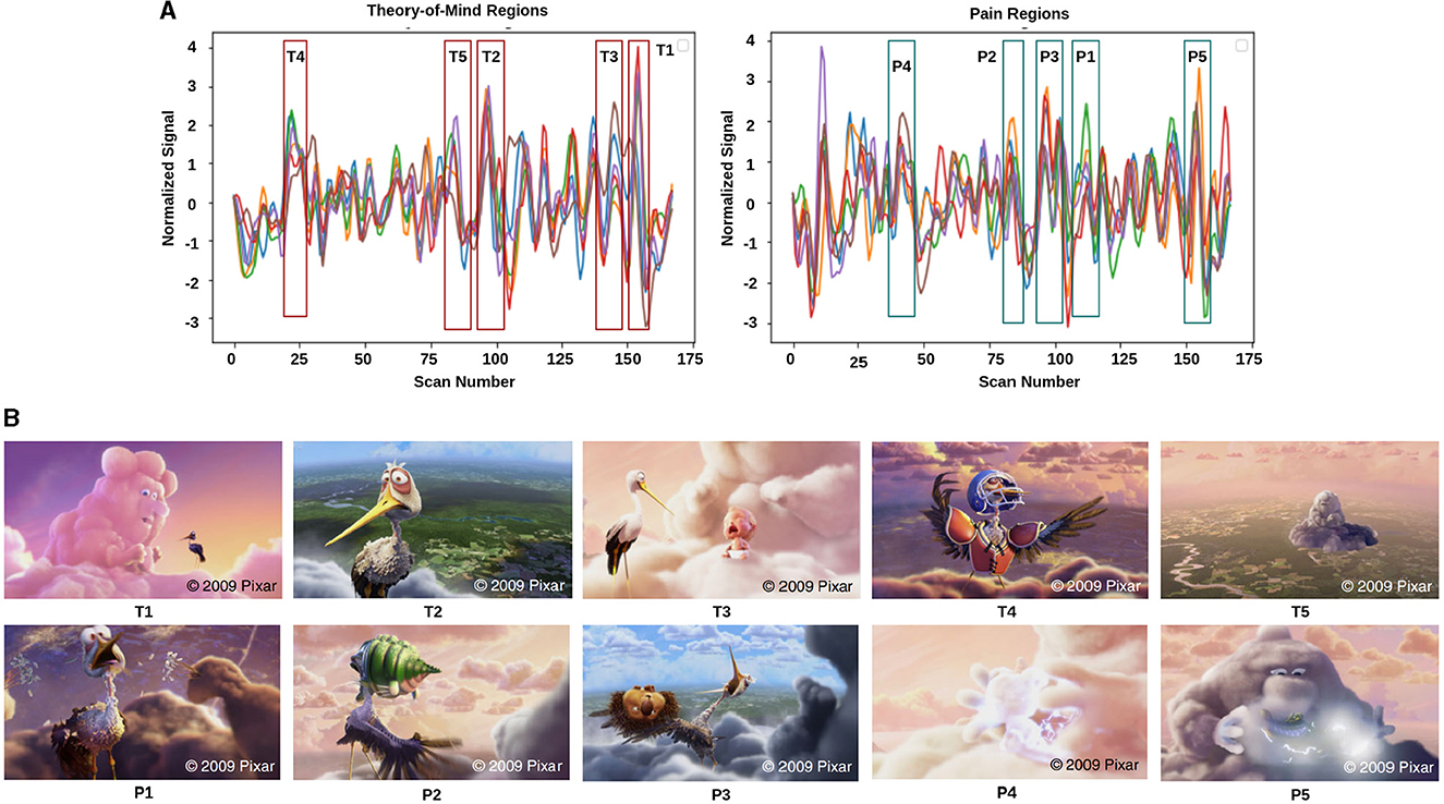
Figure 2. Movie demonstration: (A) response magnitude that evoked maximum activation in ToM and pain networks. (B) depicts the movie scenes with higher activation. Ti∈[T1, T2, T3, T4, T5] is representing ToM scenes, and Pi∈[P1, P2, P3, P4, P5] is representing pain scenes with higher activation.

2.2 fMRI data analysis and extraction of feature sets

The film features two main characters, Gus, a cloud, and his stork friend Peck, experiencing bodily sensations (notably physical pain) and complex mental states (such as beliefs, desires, and emotions). The depiction of these experiences–categorized into pain scenes and Theory of Mind (ToM) scenes–serves to investigate the viewers' brain networks that are activated during the understanding of physical and emotional states. These scenes effectively highlight the developmental changes in neural circuits involved in percieving others' physical sensations and mental conditions. Based on previous studies, we selected twelve regions of interest (ROIs) six from the Theory of Mind (ToM) network including bilateral Temporoparietal Junction (LTPJ and RTPJ), Posterior Cingulate Cortex (PCC), Ventral and Dorsal-medial Prefrontal Cortex (vmPFC and dmPFC), and Precuneus, and six from the pain network comprising bilateral Middle Frontal Gyrus (LMFG and RMFG), bilateral Insula, and bilateral Secondary Sensory Cortex (LSSC and RSSC) (Mazziotta et al., 1995, 2001; Baetens et al., 2014). A spherical binary mask of 10 mm radius was applied around the peak activity within these ROIs during specific scenes, from which we extracted time-series signals as detailed in Table 1. The selected scenes were chosen for their ability to elicit the strongest responses in the ToM and pain networks at specific time points, as illustrated in Figure 2 and Table 2. Similar to the the main study of the dataset, we extracted short-duration time-courses corresponding to peak events–five each from ToM and pain scenes, yielding a total of ten time-courses and 168 time-points. Finally, we calculated FC and ISFC as separate feature sets (Refer to Figure 3).

1. Resting state-functional connectivity: To calculate functional connectivity matrices for each participant for different time courses, we calculated Pearson's correlation between the average time series BOLD signals that were extracted from each of the spherical brain regions.

2. Computation of inter-subject functional correlations: ISFC has been used to characterize brain responses related to dynamic naturalistic cognition in a model-free way (Simony et al., 2016; Kim et al., 2018; Lynch et al., 2018; Demirtaş et al., 2019). ISFC assesses the region-to-region neuronal coupling between subjects instead of intra-subject functional connectivity (FC), which measures the coupling inside a single participant (Hasson et al., 2004; Nastase et al., 2019). ISFC delineates functional connectivity patterns driven by extrinsic time-locked dynamic stimuli (Hasson et al., 2004; Simony et al., 2016; Xie and Redcay, 2022). We calculated ISFC to check the coupling between ROIs across all the subjects.

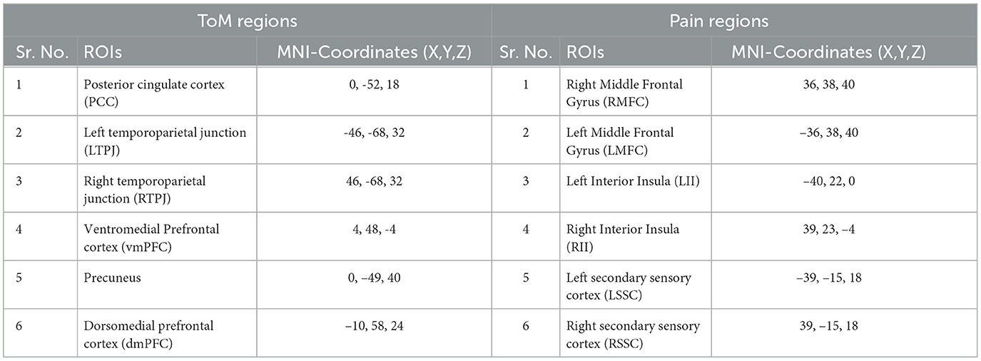
Table 1. ToM and pain brain regions and corresponding MNI-coordinated for extracting time-series signal.

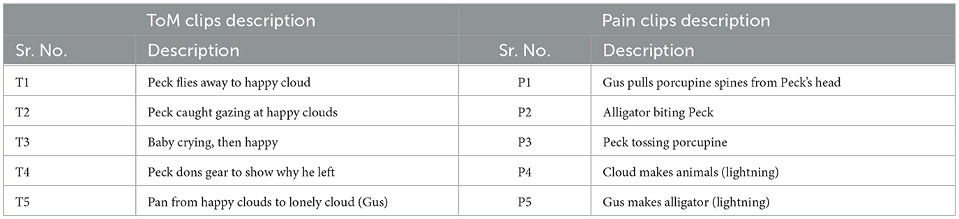
Table 2. Description of movie-clip events with higher activation for ToM and pain networks.

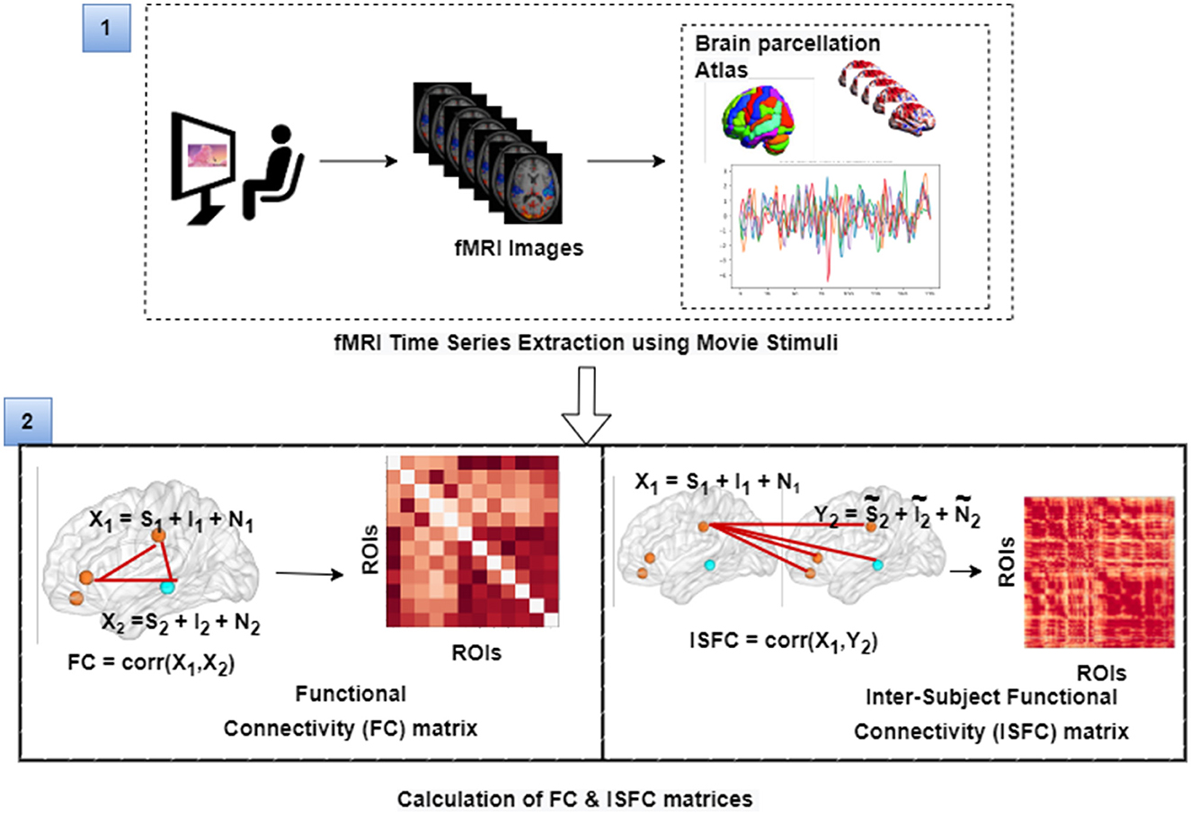
Figure 3. The figure illustrates the calculation of FC and ISFC matrices from movie-watching fMRI data that has been further used as input for decoding of cognitive state and prediction of individual performance in false-belief task purpose. Here, S represents task-evoked brain activity; I represents intrinsic brain activity; N represents noise.

2.3 Decoding of states using explainable spatiotemporal connectivity based graph convolutional neural network

We hypothesized that stimulus-driven brain features, ISFC, could decode cognitive states (ToM and Pain) more accurately than FC features. To check our hypothesis, we implemented the Explainable Spatiotemporal connectivity-based Graph Convolutional Neural Network (Ex-stGCNN) approach to classify states evoked during watching stimuli. In previous work (Richardson et al., 2018), the author applied reverse correlation analysis to average response time series to determine points of maximum activation in ToM and pain networks. We accordingly selected five-time courses (>8 sec), from each ROI, of maximum activation in ToM and Pain networks (total of ten-time courses) (Refer to Table 2). Then, we extracted time-series and converted it into a 2D matrix T*N format for each individual where T = no. of time steps, and N= no. of regions. We calculated FC matrices of size 12*12 for each time course (10 matrices for each individual) and the same for ISFC matrices. Finally, we trained our Ex-stGCNN model in two different ways: (a) using FC matrices and (b) using ISFC matrices.

2.3.1 Proposed architecture

Using PyTorch and PyTorch Geometric, the proposed model was developed in which, for every node, the Scalable Hypothesis tests (tsfresh) algorithm was used for statistical feature extraction (Kipf and Welling, 2016; Fey and Lenssen, 2019; Paszke et al., 2019; Saeidi et al., 2022). Using the FRESH algorithm concept (Christ et al., 2016), the tsfresh algorithm combined the elements from the hypothesis tests with the feature statistical significance testing. By quantifying p-values, each created feature vector was separately analyzed to determine its relevance for the specified goal. Finally, the Benjamini-Yekutieli process determined which characteristics to preserve (Benjamini and Yekutieli, 2001). We utilized node embedding methods to extract the high-level features associated with each node. We implemented Walklets and Node2Vec node embedding algorithms to observe node attributes from graph (Grover and Leskovec, 2016; Perozzi et al., 2017). Three convolutional layers were used in the proposed Ex-stGCNN model, where every layer had 300 neurons. The Rectified Linear Unit (ReLU) and batch normalization layers were implemented between each CNN layer to speed convergence and boost stability. After each CNN layer, dropout layers were applied to decrease the inherent unneeded complexity and redundant computation of the proposed multilayer Ex-stGCNN model. The final graph representation vector was calculated by applying a global mean pooling layer (Refer to Table 3 and Figure 4).

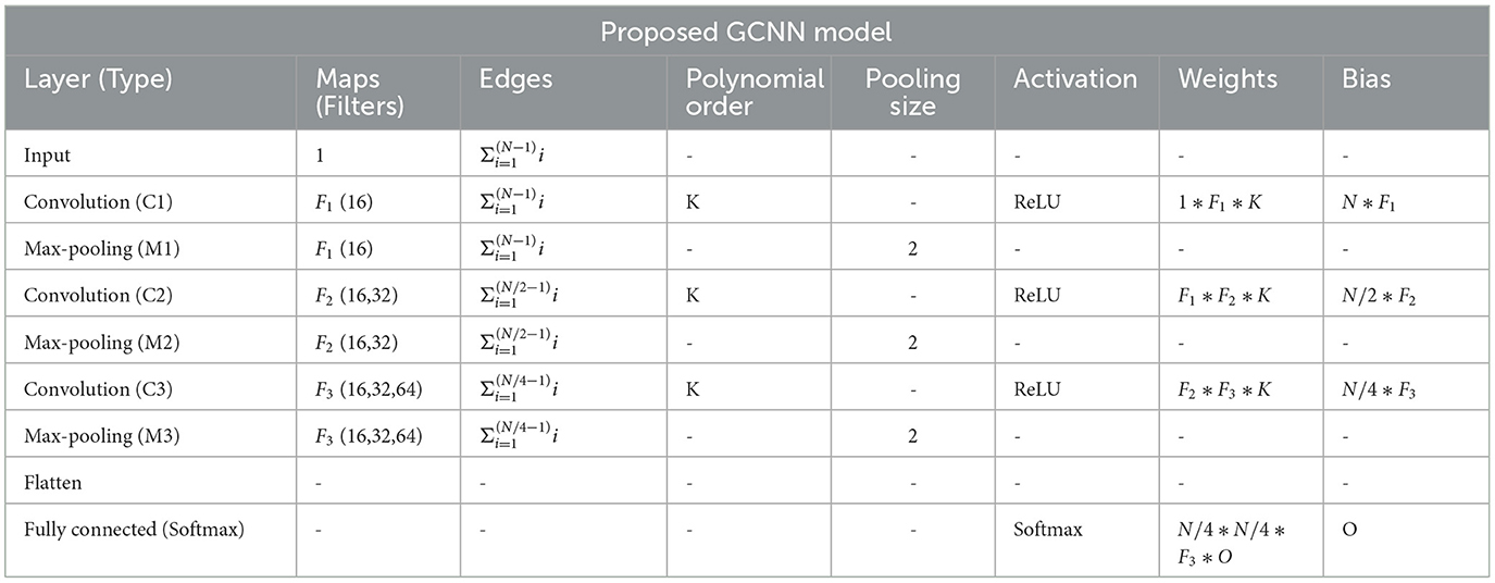
Table 3. Table shows an implementation of the proposed GCNN model architecture, where O = no. of task, N is = input size, Fi∈[F1, F2, F3] = no. of filters at ith graph convolutional layer, K = polynomial order of filters.

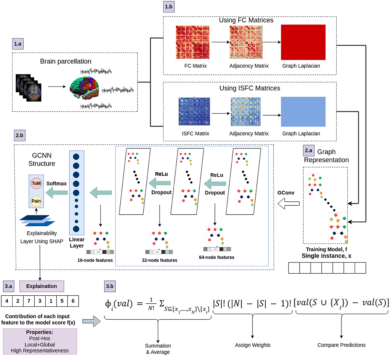
Figure 4. The architecture of proposed Ex-stGCNN model. Firstly, FC and ISFC matrices are converted into adjacency matrices and then into graph Laplacian. Finally, the graph representation of these matrices is provided as input to the model for training. We trained this proposed model using FC and ISFC matrices separately. The SHAP approach is used to extract neurological brain fingerprints to check the contribution of each brain region in the prediction.

The mathematical formation of the proposed architecture is as follows: A graph G = (V, E) consists of a set of nodes (v1, v2, ...., vn) and edges such that Eij = (vi, vj)∈E and E⊆V×V. Here, the edge has two end-points, i.e., vi and vj, which are connected through e and also refer as adjacent nodes. For developing Graph Neural Network f(X, A), where X is representing feature matrix of the nodes in the graph and A is indicating adjacency matrix, we considered spatiotemporal connectivity-based multilayer Graph convolutional neural network using Equation (1) that indicated forward propagation rule (Kipf and Welling, 2016):

Hl+1=σ( D-1/2 D-1/2HlWl)    (1)

Where A denotes adjacency matrix i.e. A+I for undirected graph G, whereas Dii = ΣjAij and Wl are a layer-specific trainable weight matrix. σ(.) denotes an activation function, such as the ReLU(.) = max(0, ). Hl∈RN×D is the matrix of activation at lth layer.

2.3.2 Spectral based GCN

We consider spectral convolutions on graphs (GCNs), which are defined as a signal's multiplication x∈RN by a filter gθ = diag(θ) using Equation (2). The graph Laplacian's eigen-decomposition in the Fourier domain was calculated via spectral GCNs using the Laplacian matrix (Kipf and Welling, 2016).

gθ⋆x=UgθUTx    (2)

Where U denotes eigenvector matrix of normalized graph Laplacian L = I−D−1/2AD−1/2 = UΛUT, and UTx denotes transformation from graph Fourier to a signal x. gθ represents function of the eigenvalues of L.

Due to the multiplication with eigenvector matrix U is O(N2), which is a complete matrix with n Fourier functions, this procedure is computationally expensive. To avoid quadratic complexity, the authors in Yan et al. (2019) suggested the ChebNet model, which ignores the eigendecomposition by utilizing Laplacian's learning function. The filter gθ is estimated via the ChebNet model using Chebyshev polynomials of the diagonal matrix of eigenvalues, as illustrated in Equation (3):

gθ ′⋆x≈∑k=0Kθk ′TkΛ~    (3)

Where diagonal matrix Λ∈[−1, 1] and Λ~=2λmaxΛ-I. λmax indicates largest eigenvalue of L, θ′∈RK = vector of Chebyshev coefficients. Chebyshev polynomial is denoted as Tk(x) = 2xTk−1(x)−Tk−2(x) with T0(x) = 1 and T1(x) = x. We calculated convolution of signal x with gθ′ filter using Equation (4) (Kipf and Welling, 2016):

gθ ′⋆x≈∑k=0Kθk ′Tk(L~)x    (4)

Where L~=2λmaxL-I, and λmax defines greatest eigenvalue of L.

2.3.3 Training and testing

We trained our model on FC matrices and ISFC matrices separately. In current study, the dataset was divided using an 80:20 ratio, and this process was carried out in a random yet controlled manner to ensure non-overlapping subsets (Rácz et al., 2021). The following steps were undertaken to split the data:

1. Random Shuffling: The dataset D consisting of N subjects was randomly shuffled to eliminate any inherent ordering.

2. Splitting: The shuffled dataset was then divided into training and testing sets using an 80:20 ratio. Specifically, the first 80% of the data (after shuffling) formed the training set Dtrain, and the remaining 20% formed the testing set Dtest.

Mathematically, this can be represented as follows:

• Let D = d1, d2, ..., dN be the dataset with N subjects.

• After shuffling, the dataset becomes D′=d1 ′,d2 ′,...,dN ′, where D′ is a permutation of D.

• The training set Dtrain is defined as Dtrain=.

• The testing set Dtest is defined as Dtest=.

To ensure robustness and avoid any potential bias from a single random split, we repeated this process 10 times, each time with a new random shuffle of the dataset. This procedure ensures that the subsets are non-overlapping across different splits, and the performance metrics reported in our results are averaged over these 10 independent splits.

We used learning rate = 0.001, dropout = 0.65, and weight decay = 0.0, patience = 3 (Saeidi et al., 2022). As batch size is one of the most crucial hyperparameters to tune, a set of batch size values was also considered. This study was implemented using an Adam (Adaptive Moment Estimation) optimizer with batch sizes of B = [16, 32, 64] across 100 epochs. For the final prediction, we used the Softmax activation function using Equation (5):

Softmax(y^i)=exp(y^i)Σi=1Oexp(y^i)    (5)

Where, ŷi∈[ŷ1....ŷO] represents predicted probability of ith task. Additionally, the optimization function was run using cross-entropy loss using Equation (6):

Loss=−Σi=1Oyilog(y^i)+ρ2NP∥W∥2    (6)

Where yi indicates targetted tasks, W represents network parameters, NP represents no. of parameters, and ρ indicates weight decay rate. To validate the results, we also implemented five-fold cross-validation.

2.3.4 Identification of neurobiological features and analysis using five-fold cross validation and leave-one-out methods

Deep learning models, particularly those involving deep neural networks, suffer from a significant black-box problem because they operate in ways that are not easily interpretable. This complexity arises due to the multiple layers and numerous parameters involved in these models. Gradient-based approaches, decomposition methods, and surrogate methods are some techniques developed to explain existing GNNs from various perspectives (Yuan et al., 2022). In the existing studies, the perturbation-based approaches were implied to identify the link between input characteristics and various outputs (Ying et al., 2019; Schlichtkrull et al., 2020; Yuan et al., 2021). However, in decoding applications, none of these techniques can guarantee the discovery of plausible and comprehensible input characteristics from a neuroscience standpoint.

In this study, the SHAP (SHapley Additive exPlanations) feature diagnostic technique was used to determine the neurological features that contributed most to Decoding of cognitive states, also referred to as dominant brain regions. The SHAP value for a feature is calculated as the average marginal contribution of that feature across all possible feature subsets. Specifically, the SHapley value for feature i is computed by summing the contributions of i in each subset S, where S does not contain i. The contribution of i is measured by the difference in model predictions when i is included and when it is excluded from S, appropriately weighted to account for the different sizes of feature subsets. We applied SHAP approach using Equation (7).

ϕi(v)=1N!∑S⊆xi,..,xN∖xi|S|!(|N|−|S|−1)![val(S∪(Xi))−val(S))]    (7)

Where: N represents all possible subsets, S is a subset of features that does not include feature i, S represents the number of features in subset S, N is the total number of features, val(S∪(i)) is the model prediction when feature i is added to subset S, and val(S) is the model prediction for subset S without feature i. To reduce the chance of bias and report low variance, we implemented a five-fold cross-validation method to evaluate the models performance (precision, recall, accuracy, F1-score) and the leave-one-out method to see performance of the model at individual level.

2.4 Prediction of individual performance in false-belief task using explainable convolutional variational autoencoder model

In a previous study (Richardson et al., 2018), the authors conducted a ToM-based false-belief task for the 3-12 yrs age group after fMRI scanning and divided all participants into three groups, i.e., pass, fail, and inconsistent, based on their performance. The previous studies (Li et al., 2019a,b; Finn and Bandettini, 2021) reported an association between brain signals and behavioral scores in resting state and during movie-watching stimuli. We hypothesized that FC and ISFC between brain regions could predict individual performance in false-belief tasks. To check our hypothesis, we used a developmental dataset with 122 participants in which the age range varies from 3–12 yrs, comprising 84 passers, 15 failures, and 23 inconsistent performers. We conducted this analysis in three ways: (a) including all 12 brain regions; (b) including dominant brain regions (Total of 8); and c) including only six ToM regions. After decoding cognitive states from FCs and ISFCs, we identified brain regions that contributed the most to prediction also referred as dominant brain regions. There were three dominant regions from ToM networks and three dominant regions from pain networks, overall six regions from ISFC-based analysis and six regions from FC-based analysis. As there was an overlap between the set of regions across analysis-type, we ended up with 8 dominant regions in total. Finally, we proposed an Explainable Convolutional Variational Auto-Encoder model (Ex-Convolutional VAE), in which we provided FC and ISFC matrices of each participant as input and performed prediction of individual performance in false-belief tasks and categorized them into pass, fail, or inconsistent groups. Ex-Convolutional VAE model included two components: (1) an encoder, which transforms the original data space (X) into a compressed low-dimensional latent space (Z), and a decoder, which reconstructs the original data by sampling from the low-dimensional latent space. (2) Use of latent space for prediction using ADAM optimizer.

The proposed Ex-Convolutional VAE model included 2D convolutional layers with ReLU activation function followed by flattening and dense layers with ReLu activation (kernal:3, filters: 32, strides: 2, epoch: 50, latent dimension: 32, no. of channel: 1, batch size: 128 for training Ex-Convolutional VAE and 32 for prediction, padding: SAME, activation function: ReLU for training and sigmoid for prediction) (Refer to Figure 5 and Table 4). The dense layer was used to produce an output of the mean and variance of the latent distribution. Using the reparameterization technique, the sampling function used mean and log variance to sample from latent distribution. The decoder architecture included a dense layer followed by a resampling layer, and 2D transposed convolutional layers with ReLU activation function. We used mean squared error (MSE) and Kullback-Leibler (KL) techniques to calculate the loss. The reason for using KL was its ability to regularize learned latent distribution to be close to standard normal distribution. We used trained Ex-Convolutional VAE Latent space for training prediction model with ADAM optimization technique. We performed the prediction using the sigmoid activation function and binary-cross entropy to calculate the loss function (epochs: 50).

Figure 5. Architecture of proposed Ex-Convolutional VAE model for predicting false-belief task-based pass, fail, and inconsistent groups. The proposed architecture first used the 2D convolutional approach to create a 32-dimensional latent space and trained the prediction model using the ADAM optimization approach (a 32-D latent space was used to train the model). The SHAP approach is used for the explainability of the proposed model.

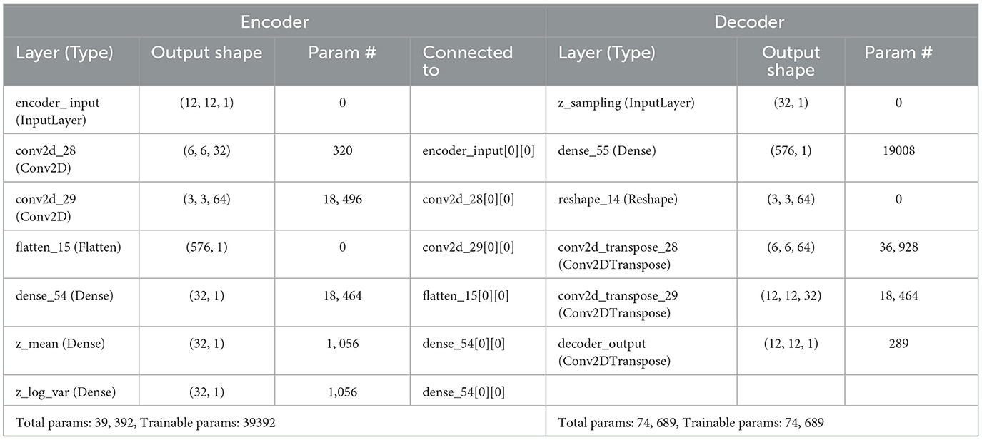
Table 4. Table shows proposed architecture of ex-convolutional VAE model and the parameters with values that have been used on it.

2.4.1 Proposed approach

In a variational autoencoder model, the encoder produces latent space from a given input while the decoder produces output from this latent space. The decoder inferences that the latent vectors have a normal probability distribution; the parameters of that which are the mean and variance of the vectors, calculated using