Digital twins are virtual representations of systems that interact with the physical system bi-directionally (Lal et al., 2020a). With the increasing availability of electronic health records and sensor-derived patient data, digital twins hold significant potential in the healthcare sector. In particular, digital twin technology enables the creation of computerized replicas of patients, allowing simulation of diverse clinical scenarios and testing of interventions in silico without subjecting real patients to avoidable risk.

A virtual patient is a digital model able to be identified from relevant bedside data and provides prediction in response to modeled inputs. Previous works have demonstrated that virtual patient simulations can be successfully utilized to train medical professionals across an array of specialties (Kononowicz et al., 2019; Lee et al., 2020; Lee and Lee, 2021; Wu et al., 2022). However, many of the previously introduced virtual patient simulation models progress only along a limited number of hand-crafted or predetermined pathways, such as looped, serious branch games, and linear text-based scenarios (Berger et al., 2018). Other examples include virtual patient simulations that progress along decision trees (Hwang et al., 2022), and another recent work (Goldsworthy et al., 2022) utilized a commercial virtual patient simulation application, First2Act, which supports only seven simulation scenarios. Although such simulation architectures have been effectively utilized to train medical professionals, they are hard to scale as each new scenario must be crafted by hand.

Recently, computational simulation models have been proposed, which seek to dynamically model the evolution of organ systems within the human body. One such simulation focused specifically on modeling how the cardiovascular system evolves based on a set of time-varying, simultaneous differential equations (Burkhoff and Dickstein, 2024). Another example is glycemic control, and there have been multiple metabolic system models based on decades of research (Chu et al., 2023). Glycemic control protocols have been optimized using these models. In addition, virtual patient models to predict lung mechanics evolution with changing ventilator settings (mechanic ventilator models) are critical to effectively managing acute respiratory symptoms for critically ill patients, but the scope of the models is very limited (Zhou et al., 2021). These models focus primarily on the one organ system and are developed based on medical, physiological, or biological knowledge, i.e., physics-based models.

In summary, digital twin applications on virtual patient modeling have gained success in modeling individual organs for drug discovery and precision medicine (Venkatesh et al., 2022; Moingeon et al., 2023), but these models rely on the full characterization of the biological and physiological functions at the cell level or the organ level. From bench to bedside, it is important to understand how the organ systems interact and orchestrate the patient’s health. For critically ill patients, the capability of modeling and predicting patient trajectories under different treatment regimens would greatly support clinical decision-making, improving patient safety and health outcomes. However, our current knowledge about the human body does not allow us to accurately depict all organ system functions using physical or mechanical models (Rovati et al., 2024). There have been emerging efforts to develop patient or human digital twins based on predictive modeling using AI and machine learning (Vallée, 2023; Katsoulakis et al., 2024; Laubenbacher et al., 2024). Despite having superior predictive capacity, the interpretability of these models is typically limited. Meanwhile, graphical models of the biomarkers of each major organ system would allow us to encode essential interactions among these biomarkers and allow for good interpretability for educational purposes and practical clinical bedside use.

Alternatively, our preliminary work (Trevena et al., 2022) proposes a virtual patient simulation architecture driven by graph-based models and focuses on patient-level simulation, i.e., modeling of the evolution of the virtual patient, determined by directed acyclic graphs (DAGs) depicting the complex pathophysiological interactions that occur within the human body. This graph-based modeling provides a more accurate and transparent presentation of complex relationships between multiple variables in a complex adaptive system where the data is often characterized by intricate interdependence and association. The improved transparency and interoperability in return ensures that the underlying expert rules building upon which the DAGs are crafted can be validated using patient data. It also allows for better visualization of variable relationships and the reasoning behind the model’s decision output. The modular and flexible nature of the graph-based model also provides an opportunity to independently and iterative refine different organ systems (respiratory, cardiovascular, neurological, etc.) as discrete models to improve efficiency, and to create a more streamlined approach to incorporate new knowledge in a specific organ system without overhauling the entire model.

The goal of this research is to develop a new highly scalable full-stack architecture for a cross-platform patient simulation application driven by graph-based models, and to present a proof-of-concept of the proposed architecture to illustrate its viability. To realize the graph-based virtual patient simulation at scale, we prioritize a highly reliable, fault-tolerant, and maintainable architecture. As we aim to develop the application as a bedside decision-support tool for clinicians in actual clinical settings, the application needs to adapt swiftly and efficiently to fluctuating user demand, and to accommodate a wide range of user devices including laptops, tablets, and smartphones with diverse operating systems (iOS, Android, etc.). Our proposed architectural approach addresses these needs in an integrated manner, contributing a sustainable and practical solution to the field. Specifically, the architecture comprises three core components: a cross-platform front-end application that clinicians and trainees use to run the simulation, a cloud-hosted simulation engine that performs all the necessary computations for each user’s simulation, and a graph database that hosts the graph model used by the simulation engine to drive each simulation. By integrating these elements, we present a highly-scalable full-stack simulation application architecture, which effectively addresses the identified challenges and paves the way for a new paradigm in patient simulation and dynamic system simulation based on graph models. Although the application focus of this paper is on modeling a virtual patient, the architecture presented in this paper could be adapted to support other dynamic systems such as mechanical, physical, and physiological systems that are graph-based, e.g., Sanchez-Gonzalez et al. (2018); Tu et al. (2019); Yang et al. (2021).

In the following sections of this paper, we elaborate on how the components of our proposed architecture synergize to overcome practical challenges. We present a proof-of-concept case study demonstrating the architecture and graph model, discuss the overarching benefits of the architecture, and outline future research directions.

In addition, our proposed architecture considers the challenge of device heterogeneity and limited processing power, especially in the medical education setting. A cross-platform programming language is preferred, which allows developers to write a single codebase that can run on multiple platforms (like Android, iOS, and web), eliminating the need to write different versions of the application for each platform. In this case, React-Native (Masiello and Friedmann, 2017), a popular cross-platform programming language, has been employed.

For the overall architecture, the cross-platform front-end (written in React-Native) is separated from the back-end simulation engine (running on a serverless function in the cloud) and the graph database (running on a dedicated server in the cloud). This separation, characteristic of microservice-based architectures, has been shown to improve scalability, reliability, and fault tolerance while also facilitating maintenance and debugging tasks (Villamizar et al., 2015). Additionally, serverless functions, due to their autoscaling and developer-friendly nature, enable developers to focus on application logic, leaving resource provisioning and infrastructure management to cloud service providers (Chadha et al., 2022). An illustration of the proposed application architecture is shown in Figure 1. Below we present the details regarding the cross-platform front-end application, the graph database construction, and the simulation engine that drives the patient pathway simulation, respectively.

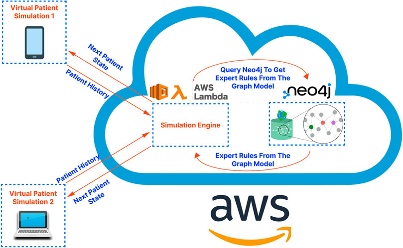
Figure 1. A high-level illustration of the proposed application architecture. The virtual patient simulations on the left-hand side of the diagram represent the front-end application. The cloud on the right-hand side of the diagram represents the cloud services serving as the “back-end” of the application. These services are hosted on Amazon Web Services (AWS) in the demo application/proof-of-concept presented in this article.

The cross-platform front-end application serves as the user interface for trainees and clinicians to interact with the virtual patient simulation by: (a) allowing users to set the initial state of the patient; (b) storing and showing the state of the patient over the course of a simulation; (c) allowing users to select interventions at each step of the simulation as desired; (d) sending the history of patient states to the cloud-hosted simulation engine to obtain the next state of the patient for the next step of the simulation (see Section 2.3 for more details); (e) tracking the relationships, i.e., edges in the graph-model that caused a change in the virtual patient’s state at each step of the simulation; (f) allowing users to connect to the graph database to visualize the relationships defined in the graph model, which influence the trajectory of the state of the virtual patient (see Figure 2 for a sample DAG).

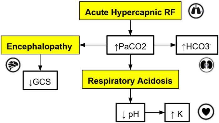
Figure 2. An example of a directed acyclic graph (DAG) depicting a subset of the interactions associated with respiratory acidosis. The boxes with a yellow background are medical concepts, and the boxes with a white background correspond to measurable patient vitals or clinical markers. PaCO2 = partial pressure of carbon dioxide in arterial blood, GCS = Glasgow Coma Scale, HCO3− = Bicarbonate.

The microservice architecture plays a crucial role here as it does not require embedding complex simulation logic into the front-end application as would be required in a monolithic application design. This division of responsibilities keeps the front-end lightweight and modular, facilitating independent development, better error isolation, and improved overall development speed.

For this application, the graph models are constructed based on expert rules. Our definition of expert rules takes into account the effects of clinical markers on each other and the causes (like interventions and interactions) that lead to certain effects on organ systems. Using a graph database, the expert rules (defined by clinicians and loaded into Neo4j via CSV files) that drive our simulation can be efficiently queried and updated. A very simple example DAG describing a subset of the interactions of organ systems and biomarkers associated with respiratory acidosis is shown in Figure 2. This DAG is constructed using rules presented in Table 1 (to be elaborated in this section).

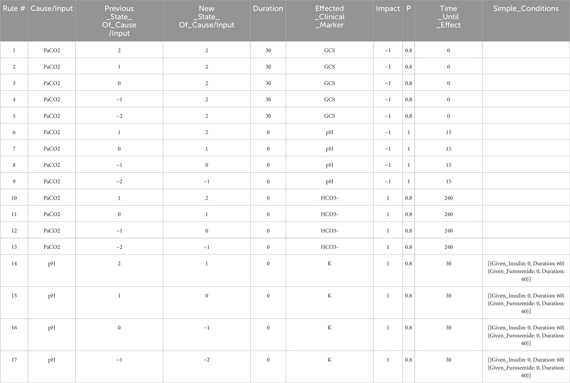
Table 1. The set of expert rules which define the edges in the Neo4j graph shown in Figure 4, and which represent the relationships shown in the DAG in Figure 2. These rules govern the progression of the state of the virtual patient described in the case study in Section 3.

Note that the simple DAG depicted in Figure 2 could be a part of a much larger DAG with many more medical concepts, measurable patient vitals, organ systems, and relationships (Lal et al., 2020b). Representing the causal pathways within the human body in an intuitive way is particularly important in a clinical setting as information overload has been correlated with an increase in medical errors (Pickering et al., 2010). Accordingly, DAGs have been utilized by clinicians in recent work to model the complex underlying causal pathways that drive the trajectory of a patient in an intuitive and visualizable way (Lal et al., 2020a). In particular, DAGs can be used to effectively model complex causal pathways within the human body as they provide a natural way to model high-dimensional directed relationships. From a simulation development perspective, instead of needing to define each new simulation scenario by hand, utilizing a graph-based simulation engine allows the number of supported scenarios to grow naturally over time as new patient vitals, clinical markers, interventions, and their associated interactions (edges) are added to the graph over the course of the iterative expert rule refinement and validation process.

The graph database utilized in this work is Neo4j (Neo4j Graph Data Platform, 2021), which has been shown to be effective at storing, querying, and analyzing graph data such as knowledge graphs (Chen, 2022). Other graph databases are also available including Amazon Neptune (Amazon Web Services, 2024) and TigerGraph (TigerGraph, 2023), among others. When developing rules for the graph model stored in the Neo4j graph database, we first define independent expert rules that have been agreed upon by the experts in the field through a formal consensus process (Gary et al., 2022). Table 1 contains sample rules expressed in the spreadsheet format to help illustrate the rule structure that is compatible with the Neo4j data structure. In the patient simulation, each rule is activated by a single triggering clinical marker or intervention (the “Cause/Input” column of the spreadsheet), and each rule causes a new incremental change or an absolute change in a single impacted clinical marker (the “Effected_Clinical_Marker” column of the spreadsheet) when all conditions for the expert rule are satisfied. Currently, states of the clinical markers are represented as integer variables (−2,-1,0,1,2) and can be color-coded in the front-end user interface. The integer values map to different value ranges of measurable biomarkers. For example, level 2 for PaCO2 corresponds to values between 71 and 120 mmHg. In the front-end application, a number randomly drawn within this range will be displayed to users, providing users with an experience closer to their regular interactions with electronic health records.

The first rule in Table 1 says, when the patient’s PaCO2 level stays at a high level (2) for a duration of 30 min, then GCS (Glasgow Coma Scale) decreases by 1 level with a probability of 0.8. In this example, PaCO2 is the “Cause/Input” of the rule, GCS is the “Effected_Clinical_Marker”, 0.8 is the “Probability”, −1 is the “Impact”, and 0 is the “Time_Until_Effect” (in minutes). The columns “Previous_State_Of_Cause/Input” and “New_State_Of_Cause/Input” describe what needs to happen to the value of the “Cause/Input” for the rule to be triggered. There are three possible triggers that we can account for: The “Cause/Input” increases, decreases, or stays at a particular value over the specified “Duration”. In this example, the “Previous_State_Of_Cause/Input” and the “New_State_Of_Cause/Input” of PaCO2 are both high (level 2), and the “Duration” is 30 min meaning that this rule is triggered after PaCO2 has been at level 2 for 30 min. By specifying a “Duration”, we can have different rules for changes that occur acutely/quickly, or which occur slowly over time. We can also model rules such as “IF PaCO2 is >70 mmHg (FOR 30 min) THEN GCS decreases” which requires that a particular “Cause/Input” (PaCO2 in this case) stays at a particular value (in this case, at a high value) for some duration. Note that, by allowing for capturing the “Duration”, the simulation is no longer memoryless and the applicability of a rule is based on the historical patient trajectory.

The effect of each rule on the impacted clinical marker is stored in the “Impact” column and is represented by one of the following integers: (−2,-1,1,2). The negative (positive, resp.) integers represent a decrease (an increase, resp.) in the value or level of the impacted clinical marker. In this example (rule #1), the GCS level will be decreased by 1 level, from its current level, and the time-lapse it needs to be effective is stored in the “Time_Until_Effect” column (with zero meaning being effective immediately in this case). To handle cases where multiple rules are simultaneously applying changes to a single clinical marker during one step of the simulation, we introduce two types of rules, one causes an incremental change, meaning that its effect is additive to others that are also incremental. The other type is “absolute”, which will override other rules once applied. In this simple example, all rules cause incremental changes.

For a rule to be activated, relevant conditions defined in the rule must be satisfied. The simple conditions are one or more independent conditions that all must be satisfied for a rule to take effect. Rules 14–16 in Table 1 have two simple conditions, and . These conditions mean that rules 14–16 will only be applied if the patient has not been given Insulin or Furosemide during the last 60 min.

Meanwhile, complex conditions are the conditions that are satisfied if at least one of a possible set of conditions is satisfied. For example, a complex condition expressed as “[,]” requires that at least one of the following must be true: (a) the patient must have no current brain swelling (b) they must have received Mannitol 30 min ago.

If all of the conditions for a rule are satisfied, we then apply the rule with the probability listed in the “P” column. The probability characterizes the chance that a certain change in the human body will occur to maintain a level of stochasticity in the simulation model.

This precise structure for expressing expert rules allows us to capture the majority of the common rules using a systematic format that is interoperable with graph databases, and enables us to customize each expert rule based on the applicability of each property.

All current and future rules can be processed in a uniform way using the same code (the code running in the simulation engine as shown in Figure 1). This means that rules in the graph database can be added and updated in the future independently without the need for the developers to write any new code. Specifically, to obtain the next patient state at each step in the simulation, the front-end application sends the complete patient history to the simulation engine and waits for a response which includes:

1. The next state (described by the states of all clinical markers) of the patient.

2. The rules that were applied (if any) which impacted the next state of the patient.

The upper and lower limits for the value of each clinical marker (currently some appropriate range between “very low” (−2) and “very high” (2)) and the lower and upper bound for each intervention (between “no intervention” (0) and “high dose intervention” (2)) are defined in the simulation engine and enforced at each step. Similarly, the length between each step in the simulation is defined (currently “15 min”).

The procedure followed by the simulation engine at each step of the simulation is outlined in Algorithm 1 and illustrated in Figure 3. This procedure integrates several functions in a modular approach to rule application and state updates.

Figure 3. Flowchart of the simulation engine algorithm.

Algorithm 1.Simulation Engine Overarching Algorithm.

Require: Time_Between_Steps=15

Require: t=0,1,…,T⊳ The steps of the simulation, each of which is Time_Between_Steps minutes apart

Require: Variable_Names=

Require: Lower_Bounds=

Require: Upper_Bounds=

Require: Patient_History=

Require: Expert_Rules←

 1: ht+1=ht

 2: InitializeSimulation (Time_Between_Steps, t, Variable_Names, Lower_Bounds, Upper_Bounds, Patient_History, Expert_Rules)

 3: for j=1to mdo

 4:   Current_Rule=Expert_Rules[j]

 5:   ApplyRules (Current_Rule, Patient_History, ht+1, Time_Between_Steps)

 6: end for

 7: for Varin Variable_Namesdo

 8:   EnforceBounds (ht+1, Var, Lower_Bounds, Upper_Bounds)

 9: end for return ht+1

To demonstrate the viability of the proposed simulation architecture, we will walk through a short case study that considers a virtual patient whose state is defined in terms of the five clinical markers shown in the DAG in Figure 2 and the corresponding nodes in the Neo4j graph in Figure 4. The trajectory of the patient will be determined by the set of edges shown in the Neo4j graph in Figure 4, each of which corresponds to an expert rule defined in Table 1. The trajectory of the patient’s state throughout this case study is summarized in Table 2, and the rules from Table 1 that were applied at each step of the simulation (each step is 15 min) are described in the “Applied Rules” column of Table 2.

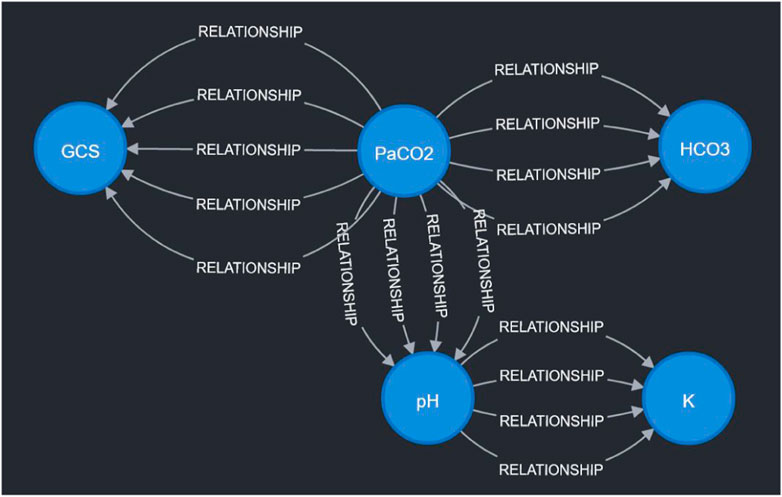
Figure 4. Visualization of sample expert rules stored in the Neo4j graph database. Each node in the graph corresponds to a measurable vital or clinical marker in Figure 2. Each directed edge corresponds to a specific expert rule in Table 1. The detailed cause-effect will be displayed when the specific “relationship” edge is clicked in the Neo4j workspace.