Source of Data

A retrospective cohort study was conducted on electronic medical record records for the derivation of 2 prediction models of 3 outcomes: mortality, hospitalization and emergency room visit. Patient collection was conducted from April 1, 2017 to December 31, 2020 and outcome assessment from January 1 to December 31, 2020. This study was approved by the ethics committee of the Alma Mater Hospital in Antioquia (INS 2022-08). The data was always managed within the Hospital with security control and passwords in the work ecosystems to protect the identity of the patients. We followed the TRIPOD-AI consensus. [7]

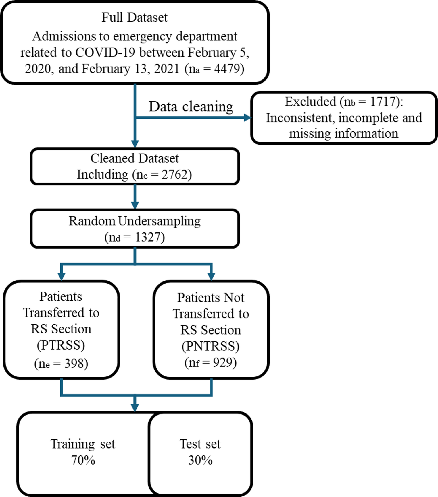
Participants

The study was carried out at a highly complex medical institution, Hospital Alma Mater de Antioquia, located in Medellín, Antioquia. This institution comprises an outpatient care facility, a home care division, and a hospital unit. Patients were eligible for inclusion if they were at least 18 years old and had at least one chronic disease as defined by the ICD-10 coding system [8] (Table 1 of supplementary appendix.). Patients were excluded if they lacked clinical data in their electronic medical records, often due to missed appointments or loss to follow-up.

Table 1 Clinical characteristics of patients included in the study cohort

Patient care followed the protocol of the “SerMás” care model, a comprehensive health management approach coordinating efforts between different health services. Importantly, the study utilized a convenience sampling method based on a contract with the healthcare payer. The cohort consisted of 5,000 patients selected in advance by the insurer according to the inclusion criteria.

Outcomes 1.

Hospital and out-of-hospital mortality: data were obtained from the GHIPS system (2024 “ALMA MATER HOSPITAL” Version: 31.2.20221216 to 37) and out-of-hospital mortality was confirmed by the health insurer and the RUAF (©information system that consolidates the affiliations reported by the entities and administrators of the Social Protection System in Colombia).

2.

Hospitalization: data were obtained on the number of times the patient consulted the assigned referral hospital or other hospitals the data was reported to the hospital when the patient was hospitalized elsewhere.

3.

Use of emergency only in the reference hospital.

Predictor Variables

We included 164 variables which were obtained from the GHIPS system, a web application that works as an electronic medical record system of the hospital in the outpatient and hospital settings. Clinical, laboratory and billing variables were extracted (Table 2 of supplementary appendix). In addition, the outcomes of mortality, hospitalization and emergency use during the evaluation year were obtained.

Table 2 Statistical analysis of Artificial neural network, XGBoost and Elastic net logistic regression models for mortality, hospitalization, and emergency room consultationSample Size Calculation

A formal sample size calculation was not made because there was a fixed cohort.

Imputation of Missing Data

A data imputation process was performed to variables with less than 20% data losses using the K Nearby Neighbors (KNN) algorithm, an imputation technique that uses information from existing data to estimate missing values. The algorithm selects a number k of observations closest to the observation with the missing value (neighbors) in the complete dataset. Then use the mean of those k neighbors to estimate the missing value. [9]

Statistical Analysis

For normally distributed variables, the mean and standard deviation are usually shown, while variables that are not normally distributed are reported with the median and interquartile range. The Hartigan immersion test was applied to describe possible multimodal distributions and the Tukey test to describe variables with distant outliers [10] DeLong’s Test, was used to define differences between model’s areas under the curve. All statistical measures were calculated with accompanying 95% confidence intervals (CIs) and w used a p-value threshold of 0.05.

Models

Three supervised learning models were used: Elastic Net logistic regression model, an Artificial Neural Network and the XGBoost algorithm. For the 3 outcomes, the database was divided into 2 parts: 85% for model training and 15% for a test dataset (Internal Validation). Before entering the data into the machine learning models, the numerical variables were centered at a mean of zero and then scaled to ensure that they all have a variance of 1. For the nominal variables, Dummies (indicator) variables (12) [11] with the ICD reference category 10 described in Table 1 of the supplementary appendix.

The Elastic Net logistic regression model is an extension of the traditional logistic regression model that uses regularization techniques to reduce the risk of overfitting, and uses a combination of the vector norm L1 (the sum of the absolute value of the elements of the vector) and L2 (Euclidean norm is the square root of the sum of the squares of the elements of the vector) for regularization, what is known as Lasso (L1), Ridge (L2) and Elastic Net (L1 and L2) regularization respectively, to automatically select the most important characteristics in the data and avoid overfitting [12].

The XGBoost algorithm is an implementation of gradient boosting with decision trees, Gradient boosting is a machine learning technique that consists of training a set of decision trees sequentially, where each tree is trained to correct the errors of the previous tree. XGBoost uses a gradient optimization technique called “stochastic gradient regularization” to adjust the parameters of individual decision trees [13].

In the neural network architecture, a feedforward model was implemented using the Keras framework. The network consisted of an input layer corresponding to the number of features in the dataset, followed by three hidden layers with 128, 64, and 32 neurons, respectively, each using the ReLU activation function. Batch normalization was applied after each hidden layer to standardize inputs and improve training stability, while a dropout rate of 0.5 was used for regularization to prevent overfitting. The output layer included a single neuron with a sigmoid activation function for binary classification. The model was optimized using the Adam optimizer with a learning rate of 0.001 and the binary cross-entropy loss function, while accuracy was tracked as a performance metric. Training was performed over 100 epochs with a batch size of 32, and early stopping was employed to terminate training when validation performance plateaued. Additional callbacks, including model checkpointing, TensorBoard logging, and a custom callback to monitor epoch-wise training times, were utilized to enhance training efficiency and transparency. Model architecture shown in suplementary sFigure 6.

For the three models all the hyperparameters were initialized randomly, a set of fitting data of these “hyperparameters” was not used and instead the 10-fold cross-validation technique was performed for each of the three models with the three outcomes, to find the best parameters between the training dataset and the validation dataset. [14] The metrics area under receiver operating characteristic curve (AUCROC), sensitivity, specificity, negative predictive value, positive predictive value and calibration curves were determined with the calculation of the slope and intercept for each outcome. For each metric, the 95% confidence interval was calculated and a maximum alpha error of 0.05 was accepted.

Models were selected for each outcome with better discrimination in AUCROC and no statistically significant differences in slope and intercept in calibration curve. The results were compared using the DeLong test for differences in the AUCROC of each of the outcomes [15].

The R programming language (version 4.2.2 Copyright (C) 2022 The R Foundation for Statistical Computing) and Python (Python Software Foundation (2021) were used. Python Language Reference, version 3.10.) to process the data and derive the model.

Risk Groups

Risk groups were created through a demo dashboard in Tableau software (Tableau. (2021). Tableau 2021.2 [Software]), in which the AI model was connected to make predictions and visualize the results in histogram form in the cohort. This allows patients to be displayed and filtered in the context of their prediction, to support decisions about the use of clinical resources and prioritization according to their risk. The dashboard creates histograms to predict the 3 outcomes with the probability extracted from the model on the X-axis and the number of patients on the Y-axis. This dashboard is the input for the end user to interact with the predictions (Fig. 1).

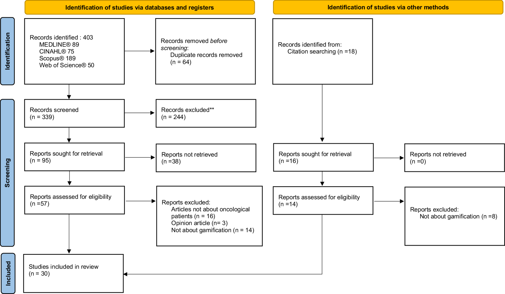
Fig. 1

Patient flowchart in the study