The concept of systematically planning experiments dates back centuries, but modern design of experiments (DoE) as a formal statistical methodology was pioneered in the early twentieth century by the British statistician Sir Ronald A. Fisher [1]. He introduced key principles of experimental design in agricultural research. From then DoE has evolved into a powerful method incorporating robust design techniques and statistical analysis to address increasingly complex experimental systems.

In the natural sciences, DoE has become an indispensable tool for empirical research, where complex systems often involve multiple interacting variables and are expensive or time-consuming. DoE has been used to optimize or improve chemical reactions in research and industry [2], pharmaceutical development [3], in synthetic biology [4], the production or recombinant proteins [5], and chromatographic analysis conditions [6], to name a few application areas in chemistry and biology.

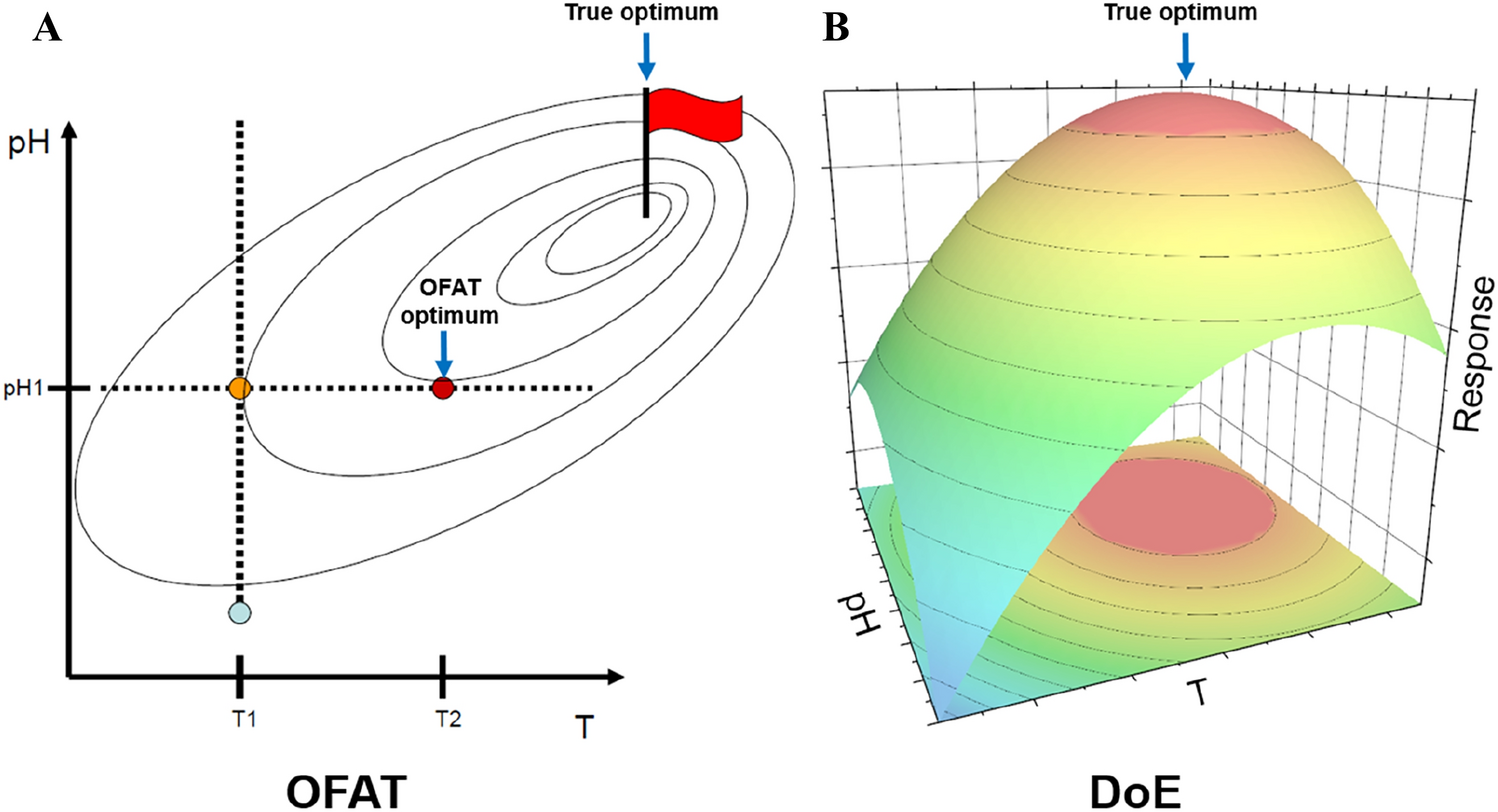
In biochemistry, systems are often highly complex, nonlinear, and sensitive to multiple factors such as pH, temperature, reagent concentrations, and incubation times. DoE is particularly well suited to such settings, where understanding these interdependencies is crucial for reproducible, reliable outcomes. One of the most common applications of DoE in biochemistry, particularly with regard to high-throughput screening in the pharmaceutical industry, is the optimization of enzyme assays. Traditionally only one factor is varied for optimization and all other influencing factors are kept constant. This one factor at a time (OFAT) approach is inefficient and often fails in complex systems to detect interactions between critical variables. If two factors interact, the response surface deviates from symmetry, which prevents the identification of the true maximum (Fig. 1a). Only step-by-step improvements are possible with lots of experiments.

a OFAT approach to optimize a system which depends on pH and T. The true optimum, indicated by the flag, is not reached by varying one parameter and keeping the other constant, if the factors interact. b DoE approach with response surface model that considers factor interactions and surface curvature

In DoE, factors that may influence a response variable are examined at least at two different levels, e.g., pH at 5.5 and 6.0. In order to investigate unpredictable interactions between the factors, different combinations of different levels of these influencing factors would have to be tested. With p factors, each with m different levels, the possible combinations very quickly take on very large numbers (mp). For example, if an enzyme reaction were dependent on six factors, such as pH, temperature, buffer salt, two cations, a detergent, and a reducing agent additive, and three different levels were tested in each case, 36 = 729 experiments would have to be carried out to cover the experimental space. This would be very inefficient and likely exceed the available resources in terms of personnel, time, and reagents. Therefore, it is mandatory to reduce such a so-called full-factorial design to less representative combinations in order to derive a multidimensional model function with which the intermediate values can be calculated (Eq. 1, Fig. 1b). The DoE approach uses specialized software to statistically reduce the number of experiments. This software enables statistical test planning and integrates data analysis. Using factorial screening designs or response surface methods, researchers can systematically vary concentrations of substrates, cofactors, buffer components, and environmental conditions to achieve dedicated precisely defined goals such as maximize enzyme activity or improve assay sensitivity or robustness.

This practical laboratory course is a continuation of a previous course about optimizing a trypsin assay for high-throughput screening of inhibitors [7]. In this course, we use two coupled enzyme reactions for the specific and quantitative detection of d-glucose. This system has a sufficient degree of complexity, which is then investigated in detail using the DoE method in two experimental cycles. In particular, factor interactions that cannot be detected using conventional OFAT approaches will be identified. The aim of the experiments is to maximize reagent savings in order to reliably detect a specific d-glucose concentration. At the same time, it should be noted that the conditions for the assay must be selected so that it is robust against pH fluctuations in the sample.

DoE enables the optimization of a complex system or process by collecting data from a limited number of experiments. This approach provides the methodological framework for structuring empirical investigations to produce valid, reliable, and reproducible results. The approach’s central objective is to obtain the greatest possible informational yield from available resources while minimizing the influence of bias and random error [8]. The principle of efficiency is not merely a matter of conserving time and materials but also generates knowledge that is deep in explanatory capacity and broad in applicability [1]. A critical aspect of this efficiency is maximizing the informational content of each experimental run. An experiment is most productive when it addresses the primary research question and generates ancillary insights that inform subsequent lines of inquiry. This is achieved by deliberately structuring treatments, carefully selecting measurement strategies, and using analytical methods that can extract multiple layers of meaning from the same dataset [9]. Scientific phenomena are rarely governed by a single factor. Rather, they emerge from the interplay of multiple factors whose effects are not simply additive. Consequently, experimental designs that vary two or more factors simultaneously provide a systematic means of disentangling these relationships. These designs allow researchers to estimate main effects, which describe the independent influence of each factor, and interaction effects, which capture how factors jointly shape the observed responses [9]. The ability to illuminate the structure of complex causal systems is one of the main strengths of modern DoE methodology. These considerations are further extended through the concept of the design space: the multidimensional region defined by the permissible ranges of all experimental factors. By exploring this space in a structured manner, researchers can characterize not only the immediate vicinity of a standard condition but also the broader operational domain within which the system exhibits stable and predictable behavior. In applied contexts, such as assay or process development, mapping the design space supports identifying robust conditions and fosters optimization and control. By deliberately integrating informational maximization, multifactorial assessment, and systematic exploration of the design space, DoE offers a coherent strategy for producing rigorous, efficient, and broadly relevant knowledge. More specifically, it is crucial that a clear goal is defined at the beginning of the optimization. Then potential influencing variables or factors must be identified, which are selected either from the literature, from personal experience, or from plausible considerations. There are two complementary approaches in experimental design. Simple 2k factorial designs and response surface designs. These designs serve distinct purposes in the progression of empirical investigation. In a 2k factorial design, k factors are examined at two levels, producing experimental runs located at the “corners” of the design space. These designs are ideal for screening because they require a minimal number of runs to estimate main effects and two-factor interactions. However, they assume a linear relationship between factors and responses, so they cannot detect or model curvature without additional experimental points. By contrast, response surface modeling (RSM) designs extend beyond the two-level framework by incorporating intermediate points, such as center or axial points, that allow for the estimation of quadratic and sometimes higher-order terms. This capability makes RSM designs especially valuable in optimization studies, where the objective is to locate optimal conditions within a defined design space rather than merely identifying influential factors. Although they provide richer predictive models, RSM designs require more experimental runs and complex analyses, making them less efficient for early-stage factor screening. In practice, these two approaches are often applied sequentially. First, a simple 2k factorial design is employed to identify the most important factors. Then, a RSM design is used to model curvature and refine the search for optimal operating conditions. This staged strategy balances efficiency with depth of understanding and aligns the design method with the investigation’s evolving objectives. If a manageable number of 2–4 factors is involved, a RSM approach is recommended.

Several experimental designs such as Box–Behnken [10], central composite [11], or mixed experimental designs have been described, which are used to create a balanced experimental design for the contribution of each factor and provide a statistically reduced number of informative trials. D-optimal designs are computer-generated designs that are made exactly for a specific problem [12]. They allow for great flexibility in how you specify your problem. They are especially helpful when you want to limit the area and there is no traditional design available. In this study, a D-optimal experimental design was chosen to achieve the number of experiments that can be performed in parallel on a microtiter plate. Experimental designs often contain a centerpoint, which corresponds to an experiment in the center of the investigated test space and which is measured several times. For efficiency reasons, it is assumed that the experimental error of the centerpoint is representative of the experimental space under investigation and provides an indication of the errors of the individual factor effects. A very important concept in DoE is the randomization of the experimental sequence to avoid external influences, such as a temperature gradient or a continuously occurring pipette error, coinciding with the effects of a factor. Of course, as with any solid data analysis, the datasets need to be curated by removing systematic and statistical outliers. Systematic outliers can result from singular pipetting errors or from effects that interfere with the measurement technique, e.g., precipitation in absorbance measurements. Statistical outliers can be recognized and excluded in the normal probability plot of the difference between the measured value and the corresponding value of the model function using the MODDE 13.1 program from Sartorius (Göttingen, Germany). Statistical outliers are defined as data points that deviate significantly from the normal probability line, which represents data points that are normally distributed around the model function. An outlier is typically defined as a data point that is more than three standard deviations from the model function. The model function describes the dependence of the response on factors and factor interactions. The latter are taken into account by the product of the factors multiplied by a corresponding parameter. In order to be able to represent curved response surfaces, quadratic terms are also included in the model function. A general model function for the factors pH and T including interaction term and quadratic terms would look as follows:

$$Y=_+_\text+_T+_\text\times T+_}^+_^,$$

(1)

where Y is the response, bx is a parameter, and pH and T are influencing factors.

The quality of a model function is evaluated with the coefficient of determination, R2, and the prediction measure, Q2:

$$^=1-\frac^_-}_\right)}^}^_-\overline\right)}^} ^=1-\frac^_-}}_\right)}^}^_-\overline\right)}^},$$

(2)

where n is the number of experiments, yi is the response of the ith experiment, \(\overline\) is the mean response, \(\widehat\) i is the fit value of the ith experiment, and \(\widehat}\)i is the predicted left-out response from the cross-validation procedure.

The coefficient of determination, R2, is a measure of how well the model function describes the data. A value of 1 means perfect agreement, which cannot be achieved experimentally, and 0 means that the data behave like noise. Q2 indicates how well the model predicts new data. Q2 is always smaller than R2. The better the model gets, the closer it gets to R2. The MODDE software offers the model validity as an additional quality criterion (Eq. 3). If this value falls below 0.25, the model has a significant lack-of-fit and the model error is significantly greater than the pure error. There are various causes of a lack-of-fit. Outliers that have not been removed can cause a lack-of-fit. Otherwise, the most likely cause is that the model is not correct and one or more important factors have to be added.

$$\text=1+0.57647 }__} >0.25 , if _ }\ge 0.05,$$

(3)

where the p value plof measures the probability that there is a lack-of-fit. If plof ≥ 0.05, the model validity exceeds 0.25 and there is no lack-of-fit. This means that the model error is not significantly larger than the pure error.

The reproducibility indicates variation in responses under the same experimental conditions. This is usually measured at the center point, located in the middle of the experimental space being investigated. With a reproducibility of 1, all replicate values are identical and the pure error is 0. Below a value of 0.5, the error is so large that the model validity cannot be evaluated any more.

$$\text=1-\frac}_}}_}}$$

(4)

$$}_=\frac^_- }_)}^ } }_}=\frac^_-\overline\right)}^},$$

with MSpe and MStot being mean of squares, which are sum of squares of the pure error (pe) and the total corrected for the mean (tot) normalized by their respective degree of freedom (n − f and n − 1, respectively), n is the number of experiments, f is the number of experiments with different experimental conditions, and \( }_\) is the mean of responses for experiments with identical conditions.

The first enzyme, glucose oxidase (GOD), enables very high analyte specificity. Even structurally closely related sugar molecules are not or only very poorly recognized by this enzyme as a substrate [13]. The d-glucose is oxidized by GOD to gluconolactone, and the oxidant oxygen is reduced to hydrogen peroxide (Fig. 2). The resulting H2O2 is simultaneously a substrate of the second enzyme, horseradish peroxidase (POD), thereby coupling the two enzyme reactions. The recognition of the H2O2 substrate is again highly specific, but many co-substrates are accepted by POD as electron donors, which predestines POD for its task as a detection enzyme. In our case, the electron donor 2,2′-azino-bis(3-ethylbenzothiazoline-6-sulfonic acid) (ABTS) was chosen because its oxidized form, a stable radical cation, has a bluish-green color and can be easily measured in an absorbance reader at 405 nm [14]. Buffer, water, enzymes, and ABTS are added for practical implementation. The reaction was started by adding the substrate d-glucose, and the measurement was carried out at 405 nm for 15 min and measurements are taken once per minute. The slope of the increase in absorbance over time serves as a readout.

Scheme of the coupled enzyme reaction used in a quantitate assay to detect d-glucose. The partial oxidation (Ox) and reduction (Red) reactions are labeled by magenta and light blue bars, respectively. In the final step, the ABTS substrate is oxidized to a stable ABTS·+ radical cation that carries a green color for detection. The crystal structures of GOD (PDB-ID: 4YNU) and POD (PDB-ID: 1W4W) are taken from the Protein Data Bank [15]

The goal of the experiment was to minimize the costs of the primary assay reagents, GOD, POD, and ABTS, while ensuring the maintenance of a robust response signal that enabled the safe detection of 0.125 mM d-glucose by using an enzyme activity model function. To this end, the lower limit of quantification (LLOQ), which corresponds to a safe detection signal at this glucose concentration, was determined in a series of independent experiments. It was defined as the mean response in experiments without d-glucose, plus five times the standard deviation, based on at least seven independent replicates. The LLOQ was determined to be 1.5 ΔE405/s × 104.

It should be noted that the experiment described here was preceded by a screening experiment with factorial design, in which the factors GOD, POD, ABTS, and pH were identified as the most influential factors. In addition, a subsequent catalog search revealed that the enzymes, and more specifically the substrate ABTS, were the most costly reagents. The factor levels in the screening experiment were chosen from typical reagent concentrations and pH values in colorimetric glucose assays: 0.1–5 U/mL for GOD, 0.1–2 U/mL for POD, 0.2–1 mg/mL for ABTS, and pH values between 5.5 and 6.5. On the basis of the results of the preceding experimental series, the ranges for these factors were chosen as follows in the first optimization round in this study: pH 5.5–6.5; GOD 0.16–0.63 U/mL; POD 0.16–0.63 U/mL; ABTS 0.09–0.38 mg/mL. In each experiment, the buffer MES was used at the same concentration of 20 mM. In addition, a constant concentration of 0.125 mM was used in each experiment. These factor ranges were selected to ensure the acquisition of reliable data for subsequent statistical analysis and to facilitate student familiarization with the methodology. On the basis of this information, a RSM design for the first experimental cycle was created using the MODDE program. The experimental design and the measured rate of bluish-green ABTS·+ radical cation are shown in Table 1. It should be noted that the experiments created patterns of factor level combinations. To avoid confounding of factor effects and artifacts caused by the patterns in the order of experiments (ExpNo), the experiments were randomized by sorting according to randomized values in the “Run order” column in Table 1. Each row of the design represented a specific experiment. These experiments were performed in a microtiter plate, and the time-dependent increase in the absorbance of ABTS·+ was measured and documented in the response column, “Rate” (Table 1). All measured rates were clearly above the LLOQ, indicating potential for further reagent savings in a second optimization round (see below). After the worksheet was completed with the measured values, the data analysis was started in the MODDE software. From then on, each evaluation figure was immediately recalculated if, for example, outliers were removed or the model function was changed. First, statistical outliers had to be removed. The experiments 1 and 2 showed a more than threefold standard deviation of the data point from the value calculated with the model function and were consequently removed (Fig. 3a). The remaining 25 data points demonstrated linear behavior in the N-probability plot, thereby indicating normally distributed residuals (i.e., the difference between the data and the model function). This is a prerequisite for conducting statistical analysis. It is imperative to emphasize that the removal of data should not exceed 10% to avoid the potential manipulation of data, which could compromise the viability of the constructed model. In the next step, the model function was reduced because many interaction and quadratic terms showed no significant effect on the response (see Supporting Information). Rigorous removal of non-significant factor and interaction terms generally increases the predictive power of the model function because possible compensating effects of these terms are prevented. This completes the optimization of the model, and the quality of the model must be finally assessed using the quality parameters R2, Q2, model validity, and reproducibility (Fig. 3d). In this case, we obtained an excellent model with a prediction measure R2 close to 1.0, a Q2 that was almost as good as R2, and an almost perfect reproducibility. The model validity was above 0.25, which indicated that there was no lack-of-fit. This was decisively confirmed by the excellent R2 and Q2 values. The highly predictive value of the model can also be seen in the perfect correlation between observed and predicted responses (Fig. 3e).

Results of first optimization round. a Normal probability plot which enables the straightforward identification of outliers from their deviation from calculated values. The residuals between the experimental and fitted values were normalized so that the units on the x-axis are equivalent to standard deviations from the model function. Outliers are indicated by dotted red circles. Each data point is labeled with its Exp. No. (Table 1). b Normalized effects on the response are shown for all significant primary factors, factor interactions, and quadratic terms, which are included in the model function. c Prediction plots are employed to illustrate the relationship between the response and the indicated primary factors. The white regions in the figure represent 95% confidence intervals. d The summary of fit plot shows the four quality parameters R2, Q2, model validity, and reproducibility. These parameters allow for a simple assessment of the model’s ability to make accurate predictions. e Observed responses are plotted against predicted responses. The strong correlation indicated a high degree of predictability for the model

The final model function contained only the factors GOD, ABTS, pH, and POD, which showed a very small factor effect, the interaction terms between GOD and ABTS, as well as GOD and pH, and one quadratic term GOD2, which indicated a curved dependency of the response from GOD concentration (Fig. 3b). The prediction graph implemented in MODDE illustrates the impact of the primary factors and also shows corresponding confidence areas that enclose a range into which newly measured data falls with at least 95% probability (Fig. 3c). The most substantial factor effect on the response was observed for GOD with a strong correlation between GOD concentration and response. This outcome was anticipated; however, the unsignificant slightly negative impact of POD proved to be a surprising revelation, since the POD reaction generated the signal. The simple explanation for this is an excess of POD activity, which is so high that even at the lowest POD concentration, the turnover of hydrogen peroxide from the GOD reaction is not limiting. Interestingly, there was a clearly significant negative effect of increasing the concentration of ABTS, which was also unexpected, since an increase in substrate concentration for POD should correlate with higher formation rate of colored ABTS·+. This unusual behavior suggested an inhibitory effect of ABTS, which has actually already been observed in the literature [16]. A physical interaction between GOD and ABTS was confirmed by the observed negative interaction between GOD and ABTS. The effect of pH on the response was also very weak. However, there was a small but significant negative interaction between the GOD factor and pH, suggesting that a deprotonated form of GOD is less active. This is in agreement with a reported pH optimum of 5.5 [14].

The learning outcomes for the students can be summarized as follows: (1) It is evident that the most significant factor effect is attributable to GOD, and this can be lowered to a considerable extent. (2) The absence of a significant factor effect (e.g., from POD) does not necessarily imply that the factor is unimportant for the assay. Rather, in our case the POD concentration was much too high, so that it did not have a limiting effect on the production of colored ABTS·+. This led to the conclusion that the POD concentration can be greatly reduced. (3) It appeared that ABTS exerted an inhibitory effect on the system, and therefore its dosage should be reduced. (4) It was evident that the pH level had a small negative effect on the response, and there was a negative interaction between pH and GOD. This suggested that when GOD loses a proton, its activity decreases.

With the aim of saving reagent costs, the ranges for the factors were changed to lower concentrations, as the lowest response from the first optimization round was still well above the LLOQ threshold of 1.5 ΔE405/s × 104. The concentrations of GOD (0.08–0.16 U/mL) and especially POD (0.04–0.16 U/mL) were drastically lowered according to the previous observations. Only pH was analyzed in the same range from 5.5 to 6.5 to investigate the previously observed interaction between GOD and pH in more detail. When the normal probability plot was used, only one outlier in 27 experiments was detected and removed. The remaining data showed a linear behavior in the normal probability plot and were therefore normally distributed. As a result of the lower concentration of the reagents, lower responses were generally obtained. Five experiments even fell below the LLOQ, so that the experimental conditions of these experiments did not fulfill the criterion of reliable glucose detection. The factor influences became smaller in the vicinity of the LLOQ and also more error-prone (Fig. 4a). As before, non-significant terms were removed to improve the model. The remaining significant terms included all individual factors, the interaction between GOD and pH, and quadratic terms of GOD and POD. The final model was again evaluated using the four quality criteria mentioned above. Although the model still showed a good coefficient of determination R2 of 0.90, the prediction measure Q2 deviated significantly from R2 at only 0.77, which indicated only moderately good predictive power (Fig. 4d). The experiment was performed technically very well, as can be seen from the reproducibility of almost 1 (0.997). However, the model validity showed a negative value, which normally indicates a lack-of-fit. However, it was suspected that the pure error of 0, which was determined from only three replicates at the center point, was not representative of the true experimental error and therefore artificially indicated a significant lack-of-fit, which may not correspond to the truth. Nevertheless, it could not be ruled out at this point that an influencing variable was not controlled and taken into account in the model. This could be the temperature, for example, which changed in the course of the experiment. The moderate predictive power is also evident in the plot of observed vs. predicted responses, where the data points scatter more strongly around the ideal line (Fig. 4b). In line with this, the 95% confidence intervals in the prediction plot around the predicted responses for GOD, POD, ABTS, and pH are also larger than in the very good model from the first optimization round (Fig. 4c). Overall, the predictive power of the model can therefore only be assumed to be moderately good, although one can make reasonable statements for the area investigated. As a result of the strong reduction in the POD concentration, its activity became limiting and showed a stronger effect on the response in the same order of magnitude as GOD. For the first time, a significant positive effect was also observed for the factor ABTS, as its inhibitory effect was no longer as strong in the lower concentration range. The negative effect of higher pH values and in particular the negative interaction with GOD was confirmed, making its activity reduction by deprotonation very likely. The negative quadratic POD term suggested that the concentration of POD passed through an optimum and the response decreased again at very high POD concentrations (Fig. 4a). The exact cause of this would have to be clarified in further biochemical experiments. An aggregation of POD would be conceivable, which could lead to a decrease in its activity at higher concentrations. In the prediction plot, the indicated minimum is probably due to a greater inaccuracy in the lower concentration range. For the most cost-effective glucose assay, the pH value 5.5 would be selected, at which the activity of the coupled enzyme system is highest. With the aim of saving reagents, the lowest tested ABTS concentration would then be used because its effect on the response in the investigated range of 0.025–0.09 mg/mL is very small. The two enzymes GOD and POD are essential for signal generation. To ensure that POD is not limiting, a concentration of 0.12 U/mL would be chosen, at which the response becomes maximal. With regard to GOD, one should not go below the artificial minimum in the prediction plot, so that the smallest GOD concentration that appears suitable is around 0.12 U/mL. We know from the first optimization round that POD is not limiting for equal GOD and POD concentrations. The MODDE software uses the model function to calculate the predicted response from each factor level combination with a lower and upper limit that defines a 95% confidence interval. For the selected factor level combination GOD (0.12 U/mL), POD (0.12 U/mL), ABTS (0.025 mg/mL), and pH 5.5, a response in the range of 2.14–2.79 ΔE405/s × 104 was obtained, which comes very close to the LLOQ of 1.5 ΔE405/s × 104, but does not fall below it, so that 0.125 mM d-glucose can be reliably detected.

Results of second optimization round. a Normalized effects on the response are shown for all significant primary factors, factor interactions, and quadratic terms, which are included in the model function. b Observed responses are plotted against predicted responses. The strong correlation indicated a high degree of predictability for the model. c Prediction plots are employed to illustrate the relationship between the response and the indicated primary factors. The white regions in the figure represent 95% confidence intervals. d The summary of fit plot shows the four quality parameters R2, Q2, model validity, and reproducibility. These parameters allow for a simple assessment of the model’s ability to make accurate predictions