Decoding extracellular recordings is an essential task for both electrophysiological studies and brain–computer interface (BCI) applications [1]. Spike sorting, which involves detecting and attributing spikes to their putative neurons1, is the first step in processing these recordings [2]. Conventional spike sorters comprise several steps, i.e. spike detection, feature extraction, and clustering.

Recently, the advancement of neural probes enables the recording of thousands of tightly-placed electrodes. For example, the Neuropixels (NPs) series (1.0 [3], 2.0 [4], Ultra [5]) are capable of recording 384 channels in parallel with electrode pitches of 20, 15, 6 um, respectively. The large number of channels causes an increase in computational workload and processing time, while the shrinkage of pitches causes higher noise levels [5] and more drifting problems [6], compromising the accuracy of the spike sorters.

Modern spike sorters [7, 8] utilize deconvolution and drift registration iteratively in time chunks to counteract the accuracy degradation. However, these techniques require more computation and struggle with high noise levels and complex neuron distributions.

With the NNs demonstrating promising performance in various fields, several studies on NN-assisted spike sorters have been conducted to replace some steps in conventional spike sorting pipelines [9, 10]. For example, YASS [9] used two NNs for spike detection and waveform denoising, respectively, each of which was constructed with convolutions on the temporal and spatial dimensions. However, because only specific steps in the spike sorting pipelines were substituted with NNs, other non-NN processing algorithms were still present, which may require manual tuning when adapting to different recordings. For example, [11] employed two NNs for spike detection and feature extraction, achieving promising results in processing 128-channel recordings. However, to improve generality, the method uses an unsupervised PCA-based clustering that requires manual determination of neighbor counts and distance thresholds. There were also NN-only designs utilizing several NNs [11, 12] or branches [13] for specific stages in spike sorting. Nevertheless, these designs were difficult to optimize for computational efficiency, since several different algorithms were involved which are hard to ameliorate collectively.

By contrast, the solutions based on end-to-end NNs, which bind the whole spike sorting pipeline into a single NN, are promising because of their simplicity and integrity. DualSort [14] demonstrated an end-to-end NN for sorting a single-channel recording by incorporating data augmentation based on temporal shifting and population-based post-processing. However, the feasibility of the design for processing recordings from high-channel-count neural probes remains unproven.

Manual annotations of neurons: because the number of output neurons varies case by case, each model requires separate training for each recording. NN training demands multiple annotated spikes per neuron, with the total annotation burden increasing with neuron count. Moreover, high-channel-count recordings require more annotated spikes per neuron to capture additional spatial patterns compared to single-channel recordings.. While few-shot training with adversarial representation learning has been used in a previous study [10], it was limited to single-channel recordings and only performed feature extraction on the NN with only tens of spikes utilized during training.

Non-parallelizable post-processing: although the NN accelerations are well-supported by parallel computation hardware (e.g. GPUs), the post-processing in DualSort [14] resists parallelization due to temporal data dependencies—output of each timestep depends on its predecessor.. Therefore, despite the NN inference could be computed in parallel, the post-processing has to be performed one step at a time, leading to excessive execution time.

To tackle the aforementioned challenges, we propose E-Sort2, a novel spike sorter utilizing an end-to-end NN trained with transfer learning and a parallelizable post-processing scheme. Our contributions are as follows:

We propose a framework of transfer learning for end-to-end spike sorting. We designed a NN with temporal and spatial filters, similar to [9]. We pre-trained these filters on large recordings and fine-tune these filters, along with training the classifier from scratch with the starting few spikes from the test recording.We designed a post-processing composed of a triangle filter followed by peak detection and thresholding for rejecting redundant spikes and suppressing false positives (noises). This post-processing is GPU-friendly and compatible with NN frameworks.We evaluated E-Sort on both synthetic and real recordings. Compared to the state-of-the-art NPs sorter Kilosort4 [7], our transfer learning strategy achieved comparable accuracy while reducing required training duration by 2.25× versus training from scratch. Our design significantly reduced execution time versus existing sorters while matching Kilosort4 accuracy. On real datasets, pretraining improved accuracy by approximately 30% versus scratch training with identical sample sizes.

We evaluated our framework using both synthetic hybrid datasets and real experimental recordings. The hybrid dataset was generated using the MEARec [15] package, which employs real biophysical multi-compartment models from the Neocortical Microcircuit Collaboration Portal to create spike templates. For our experiments, we used templates from 13 layer 5 juvenile rat somatosensory cortex neuron models. These templates were convolved with user-defined spike trains and combined with noise to generate recordings with customizable noise levels, electrode geometries (probe configurations), and drift patterns. We created multiple recordings with different parameter configurations to evaluate our design’s robustness through comparative analysis. The availability of ground truth spike trains during recording generation facilitated performance evaluation.

For real-world validation, we used publicly available chronic recordings from the left primary visual cortex of three mice. The mice were head-fixed while being presented with colored visual stimuli on three screens. From these, we selected seven recordings (AL_031_2019-12-02, AL_031_2019-12-03, AL_031_2019-12-13, AL_031_2020-01-07, AL_031_2020-01-16, AL_031_2020-02-04, AL_031_2020-02-19) from mouse 3, which was implanted with a single-shank NPs 2.0 probe.

Since obtaining ground truth for these experimental recordings is challenging, we processed them using Kilosort4, the state-of-the-art spike sorter for NPs data, with default parameters to establish reference spike trains. We retained only clusters classified as ‘good’ by Kilosort4, indicating they exhibit clear refractory periods and show no evidence of requiring further subdivision.

3.1. Preliminaries

Training NNs for spike sorting is different from that for other tasks, e.g. computer vision or natural language processing. Spike sorting extracts individual neural activities from extracellular recordings. However, the number of spike sources is a priori for every recording, and the recording devices and environments can cause significant differences in signal qualities, noise levels and various artifacts. NNs aiming at acquiring final spike trains should be tuned for every recording, which is associated with heavy labor by experienced neuroscientists to label the spikes from the recording. In this paper, we aim to reduce this labor by utilizing a pretrain-and-finetune strategy. Considering the missing of the ground truth for real recordings, we apply one widely used state-of-the-art offline spike sorter, Kilosort4 [7] to generate the spike trains for the convenience of experiments, which we consider as the golden label for training and evaluation. Note that this can be replaced with any off-the-shelf spike sorting algorithms, and in practice, these labels for training (finetuning) should be marked manually by the experts in the corresponding neuroscience experiments. We would like to clarify that, like other spike sorters with NNs [9], our design requires some labeled spikes for training, but it is dependent on any other spike sorter. Even for spike sorters without NNs, for example, Kilosort4, some priori on the targeted recording is required to tune the parameters (e.g. thresholds) for getting the optimistic performance.

3.2. Dataset preparation

To leverage both the spatial and temporal information in the recordings, we define the windows containing all probe channels within a time interval as the input for the NN. However, spikes occupy only a small fraction of extracellular recording time and the firing rates of different neurons vary significantly, e.g. excitatory cells fire several times faster than inhibitory cells. Using all windows would create dataset imbalances in both spike/non-spike ratio and spikes from different neurons, which would degrade NN performance in identifying the sparse spikes from the recording and distinguishing the putative neurons for each spike, respectively.

To increase the numbers of the spike-containing window samples and balance the number of windows with spikes from different putative neurons in the dataset, we construct the dataset through three steps: we first select windows containing at least one centered spike; secondly, the selected windows are augmented by applying temporal shifts up to with paddings from the recording, and therefore each spike appears in windows, increasing the number of spike-present samples in the dataset; finally, an equal number of non-spike windows is randomly selected from the recording, ensuring that the total number of non-spike windows matches the number of spike-present windows, thus balancing the number of spike/non-spike samples in the dataset.

3.3. Transfer learning

Transfer learning is a technique for pre-training a NN on a large dataset and fine-tuning for a new small dataset. In this paper, we employ this approach to reduce the number of annotated spikes required for acquiring a high-accuracy NN for a specific recording.

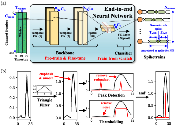
The NN architecture consists of a backbone and a classifier for feature extraction and classification respectively, as shown in figure 1(a). The backbone is constructed with two temporal filters with channel count and and one spatial filter with channel count Cs, similar to what is used in YASS [9]. These filters extract the latent features from the temporal and spatial dimensions with linear mappings on the corresponding dimensions, each of which is followed by normalization and ReLU activation for regulation and introducing nonlinearity. We pre-train the backbone on long-duration and neuron-rich recordings to find general features across different classes of spikes. The classifier containing a fully-connected layer followed by a sigmoid activation, is trained from scratch for each recording because the number of output channels is dependent on the number of neurons in the recording.

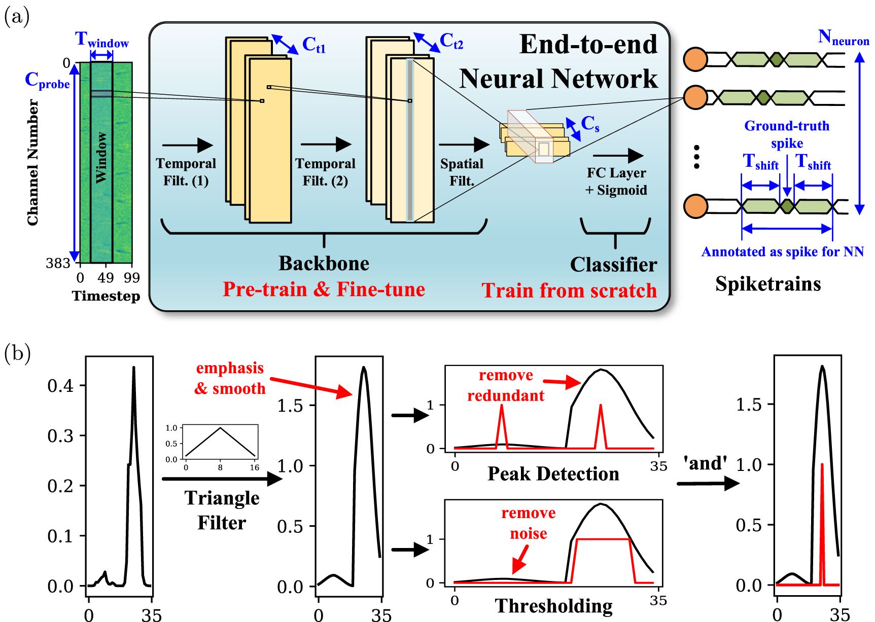
Figure 1. The proposed E-Sort spike sorting framework. (a) End-to-end NN pre-training & finetuning scheme. (b) Parallelizable post-processing for removing noises and redundant spikes.

Download figure:

Standard image High-resolution image 3.4. Post-processing

Due to the temporal shifts used in dataset augmentation, each spike should be detected repeatedly by the NN. To eliminate redundant spikes and suppress false positives (e.g. noises mis-detected as spikes), we propose a post-processing framework, which is parallelizable and compatible with modern deep learning frameworks, as shown in figure 1(b).

Considering that the noise is unlikely to produce continuous detections in the temporal dimension, and each spike should be detected continuously, we apply a triangle filter on the temporal dimension to emphasize and smooth the output from the NN. The emphasized spiketrain is subsequently processed by two algorithms. First, peak detection removes redundant spikes, which finds local maxima by comparing each data point with two temporally adjacent points. Second, thresholding eliminates noise-induced detections, which filters out the data points that exceed a certain threshold. Final spike detections are determined by points satisfying both criteria.

4.1. Experimental setup

The proposed E-Sort was implemented using the PyTorch framework. For balancing the spike-noise ratio, was set to 5. Since the implemented NN only has four layers, all training and finetuning was performed in 50 epochs under the Adam optimizers with a learning rate of 5 for rapid convergence. The batch size in training and testing of the NN were both set to 1024, while the batch size in post-processing was 10 000. The experiment platform is equipped with 32 CPU cores from the Intel Xeon Platinum 8468 CPU with 128GB physical memory and an Nvidia H100 GPU. We used the sorting accuracy to evaluate the performance of our framework, which is defined as

where , , and are the number of true positives (spikes sorted correctly), false positives (noises mis-sorted as spikes), and false negatives (spikes mis-sorted as noises) results.

4.2. Transfer learning results4.2.1. Results on hybrid recordings

The hybrid recordings were generated using MEARec with a fixed duration of 100 s. The training set was sampled from the first 50 s, while the last 50 s were used for testing. Different random seeds were applied to generate separate recordings for pre-training and fine-tuning. The training samples, either training from scratch, pre-training or fine-tuning, are coming from the first 50 s. For pre-training, all spike-centered windows are augmented and paired with randomly selected noise windows, while for fine-tuning, only a certain number of spikes per neuron sampled from the beginning part are augmented and paired with noise windows. On the other hand, the testing is always taking all samples in the last 50 s into account. The neuron densities were set to 1.5 and 1 per mm3 in pre-training and fine-tuning recordings, respectively. By default, the recording was generated with NPs 1.0 probe geometry, and the noise level was set to 10 µV, with no drifting applied.

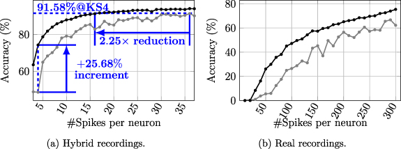
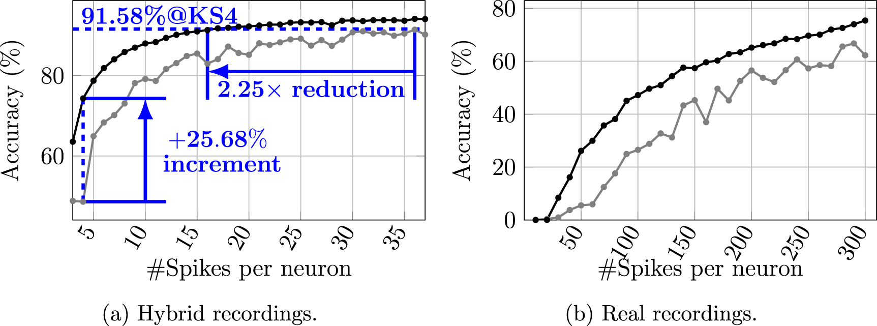
To evaluate the performance of the pre-trained model on the hybrid recordings, the pre-trained model was acquired by training with all spikes from the first 50 s of the recording for pre-training. We then assessed the accuracy achieved with various numbers of spikes per neuron for fine-tuning, which is denoted as , as shown in figure 2(a).

Figure 2. Achieved accuracy versus number of spikes per neuron for finetuning pretrained models () and training models from scratch ().

Download figure:

Standard image High-resolution image

Compared to the model trained from scratch, fine-tuning from the pre-trained model achieves up to 25.68% higher accuracy. This advantage diminishes with more training spikes for fine-tuning/training because the model trained from scratch progresses towards learning features from the increased samples, reducing the benefit of pre-learned features from pre-training. To reach comparable accuracy (<0.5% difference) with Kilosort4 (KS4), the pre-trained model only requires 16 spikes per neuron for fine-tuning, while the model trained from scratch requires 36 spikes per neuron, indicating a 2.25 × reduction in the training set.

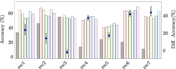
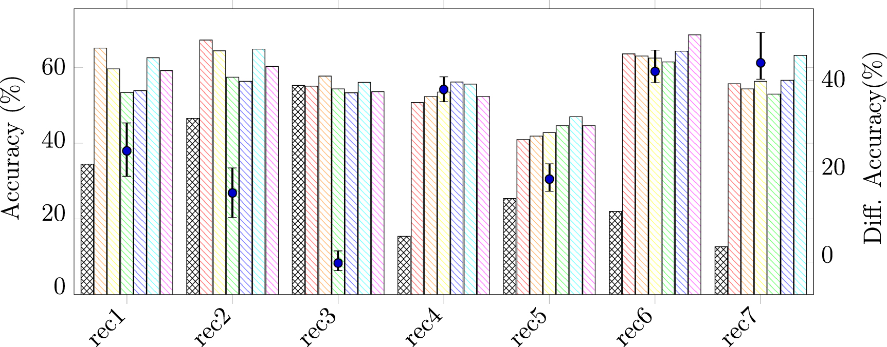
4.2.2. Results on real recordings

We evaluated our design on real NPs 2.0 recordings, as shown in figure 2(b). Because the referenced spike trains were acquired by Kilosort4, the accuracy achieved in the real recordings reflects the agreement between the framework and Kilosort4. The model was pre-trained on the first recording (AL_031_2019-12-02) and fine-tuned on the second recording (AL_031_2019-12-03). As a comparison, we also trained and evaluated the model without pre-training on the second recording. Comparing with hybrid recordings, more samples are required to achieve comparable accuracy in real recordings. However, with the same number of training spikes per neuron, the pre-training model could still outperform the model training from scratch. After evaluating each pair of 7 recordings mentioned in section 2, the pretrain-and-finetune schedule can improve the accuracy by 30% on average, as shown in figure 3.

Figure 3. Sorting accuracy achieved in real recordings. The models are obtained by either training from scratch (), or finetuning after pretraining on other recordings (rec 1: , rec 2: , rec 3: , rec 4: , rec 5: , rec 6: , rec 7: ). The min, mean, and max improvements by pretraining on different recordings are visualized ().

Download figure:

Standard image High-resolution image 4.3. Post-processing algorithm analysis

The post-processing algorithm is customized to extract the spike trains from the NN outputs. Compared to the post-processing implemented in DualSort [14], our implementation is fully vectorized and thus can be easily accelerated by GPUs. For making quantitative and fair comparison in execution time, we implemented the post-processing in DualSort in our platform and used the spike trains of the hybrid recording to reversely generate the output of their NN, i.e. the prediction group and time. We benchmarked the execution time of DualSort post-processing in both CPU and GPU, which consumed 90 s and 360 s, respectively. Because of the sequential time-step processing in DualSort, the GPU-based implementation consumed even longer time. By contrast, our post-processing implementation only consumed 1.22 s.

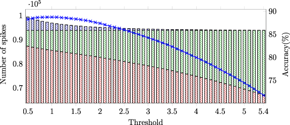
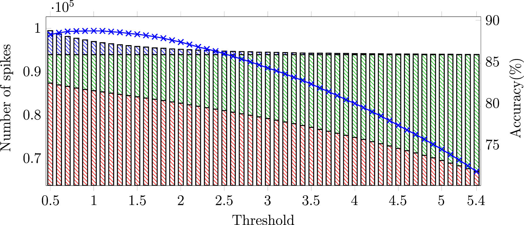
We also analyzed the hyper-parameters of the proposed algorithm. Since the peak detection has no tunable parameters, and the parameters of the triangle filter and thresholds are highly related, we kept the triangle filter with maximum amplitude as 1 and length as 17 samples, and varied thresholds from 0.5 to 5.4 in 0.1 increments to assess its impact on accuracy, as shown in figure 4. With increasing thresholds, both and are increasing and are decreasing. At lower thresholds, errors primarily originate from noise. In contrast, when the threshold is larger, the accuracy will also be decreased because truth spikes are filtered out.

Figure 4. Performance of E-Sort with different threshold in post-processing. The visualized spikes include all ground-truth spikes, which are either detected correctly (truth positive: ), or wrongly (false negative: ), along with the faulty detected spikes (false positive: ). The accuracy () is also calculated with these spike counts.

Download figure:

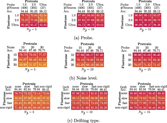
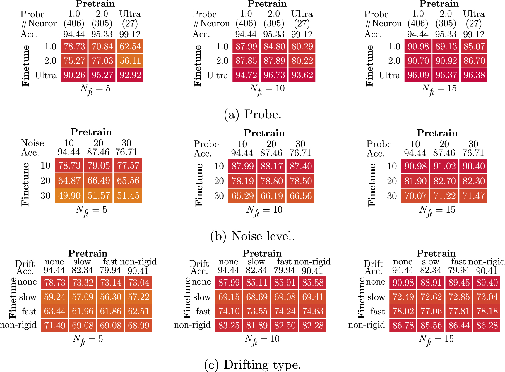
Standard image High-resolution image 4.4. Generality of pre-trained model

To evaluate the generalizability of the pre-trained models in different recordings, we performed the validations on the recordings with different characteristics, involving various probes (NP-1.0, NP-2.0, NP-Ultra), noise levels (10 uV, 20 uV, 30 uV) and drifting types (none, slow, fast, non-rigid), as shown in figure 5. The first row values show the accuracy achieved by the pretrained model in the pretraining dataset, which stands for the accuracy achievable by the model with sufficient training samples. Generally, the model have better performance when the neuron count is smaller or the side effect is weaker (low noise level/light drifting). Also, the accuracy variations among different pre-trained models on each fine-tuning recording reduce with the enlarging of , because the models learn more effectively when more samples are involved during fine-tuning.

Figure 5. Validations of recordings with different (a) probes, (b) noise levels, and (c) drifting types.

Download figure:

Standard image High-resolution image

For the probes with different geometries, there are two factors affecting the performance of fine-tuning. First, the recording from a more compact probe contains fewer neurons with a fixed neuron density. It is difficult for the model that is pre-trained with the recording containing few neurons to learn general features for various neurons, thus undermining its performance during fine-tuning. Also, because it is easier to distinguish different spikes for the recording with fewer neurons, the model training or fine-tuning for these recordings generally achieves a higher accuracy. Second, the recordings from the same probe have more similarities than those from different probes. Therefore, it is easier to transfer the knowledge when adapting to the recording from the same probe in pre-training, and this consistency can provide slightly higher performance (∼ 1%) under certain circumstances. However, when more samples are involved during fine-tuning, the pre-trained models can be generally applied to the recordings from different probes without compromising visible accuracy degradation.

As for the various noise levels, the accuracy decreases with the deterioration of the noise involved in the recording. Similarly to cross-probe testing, fine-tuning the model acquired on the recording with the same noise level can result in slight improvements, but still there is no apparent difference even when a few samples are utilized during fine-tuning.

The testing on different drifting types was conducted in four representative patterns, viz., none (no drifting), slow, fast and non-rigid. For the slow and fast drifting, all neurons are moving coherently. All drifting was applied in the z-dimension, i.e. up-and-down. In the slow drifting, the velocity was set to 10 um s−1 with a drifting range of 30 um, while the fast drifting was configured with a jump with a maximum distance of 15 um every 20 s. As for the non-rigid drifting, the neurons are drifting differently, with a velocity and range of 80 um s−1 and 10 um, respectively. The fine-tuning for the recording without drifting achieves the highest accuracy, followed by non-rigid, fast, and slow. It indicates that the model is more sensitive to the drifting range instead of the velocity, which may be because the neuron positions are learned in the NN and long-distance drifting harasses the utilization of this feature. However, similar to the aforementioned comparisons across different probes and noise levels, the models pre-trained from the recordings with different drifting types have negligible impact on the fine-tuning performance.

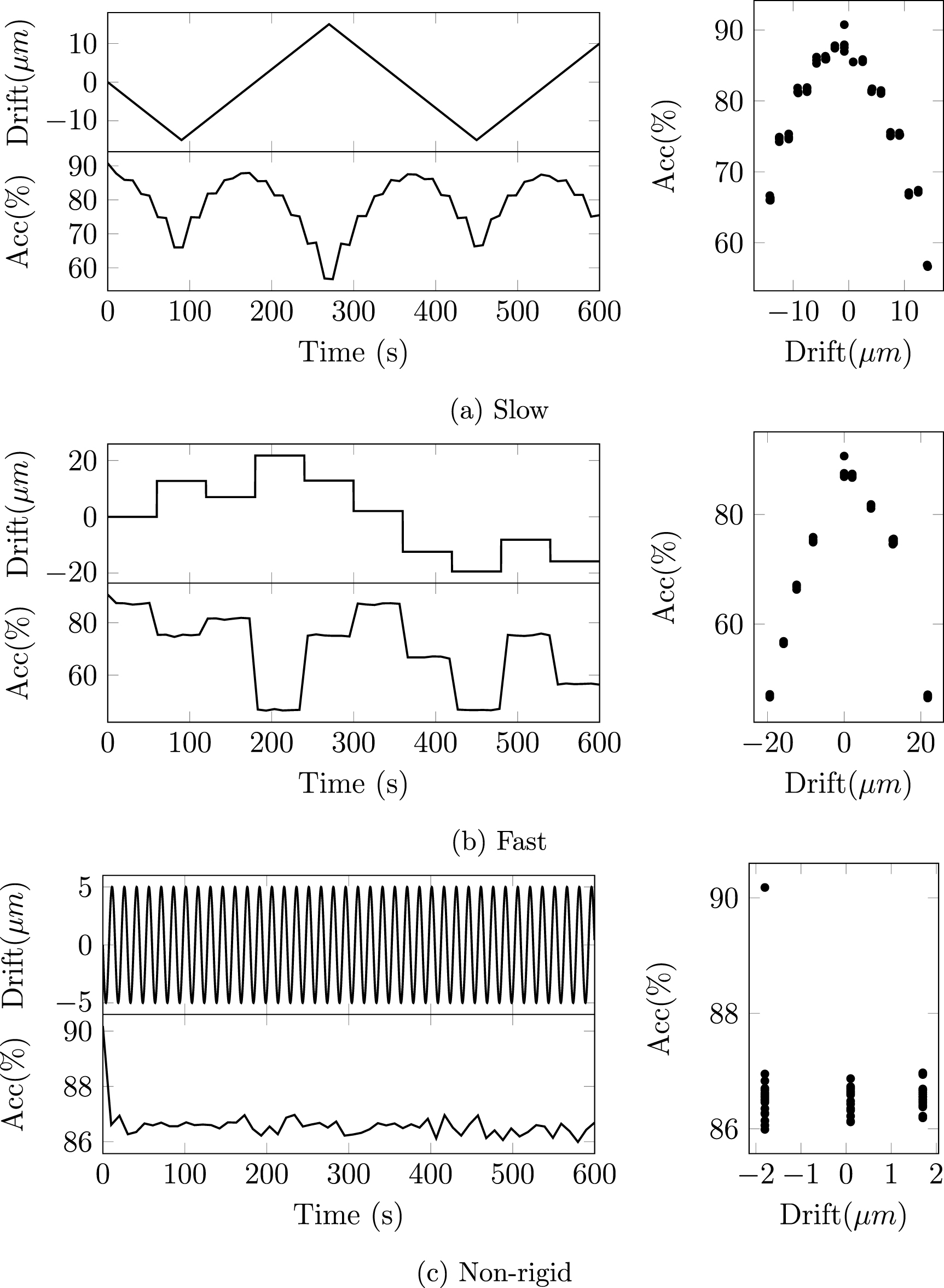
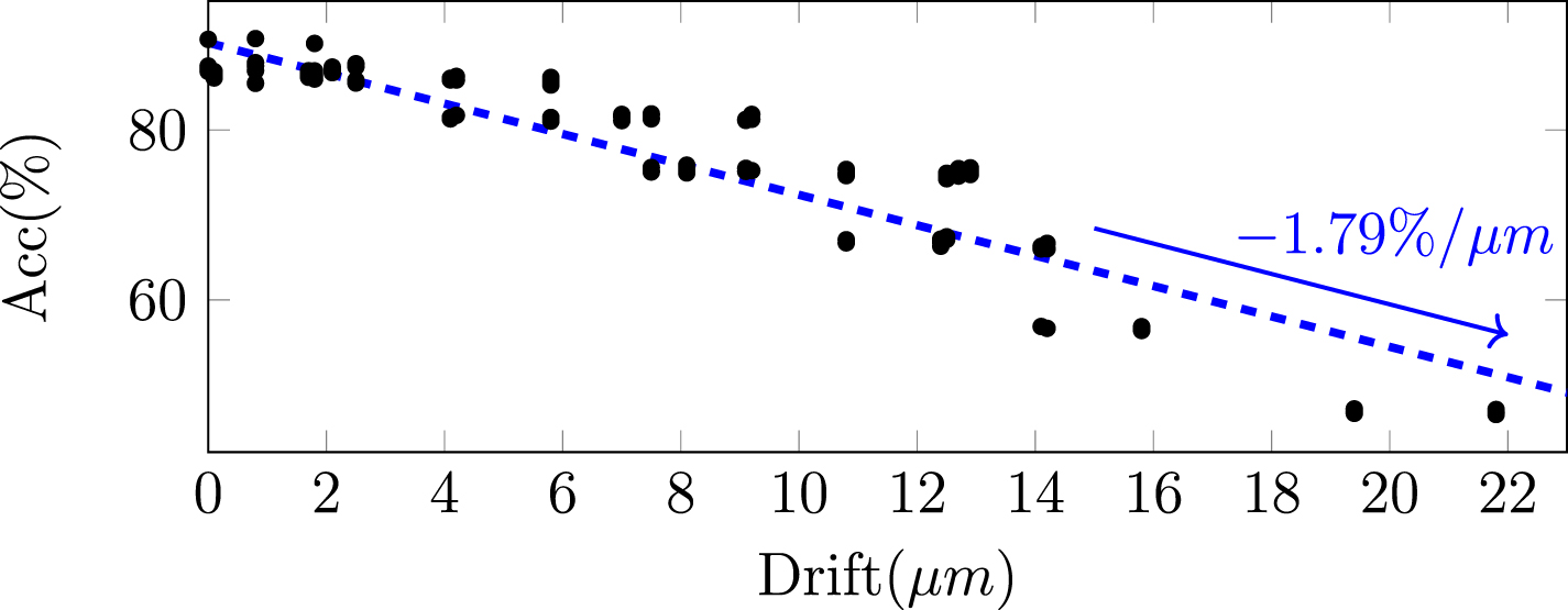
Considering that drift emerges gradually over longer timescales, we assess its impact by generating longer-duration recordings, as shown in figure 6. The three drifting patterns are generated randomly with MEARec, with the configuration described previously but with 600 s duration. The sorting accuracy is measured every 10 s. Generally, the achieved accuracy decreases approximately linearly with the increase of drifting distances. After linear regression, the averaged accuracy decrease is -1.79% for drifting distance, as shown in figure 7.

Figure 6. Validations of longer-duration recordings with different drifting patterns (a) slow, (b) fast, and (c) non-rigid.

Download figure:

Standard image High-resolution image

Figure 7. Drift distance versus accuracy reduction.

Download figure:

Standard image High-resolution image

In summary, the pre-trained model could be generalized to various probes, noise levels, and drifting types. However, a neuron-rich recording for pre-training is more favorable when a few spikes are provided for fine-tuning.

4.5. Comparisons with state-of-the-art spike sorters

We compared our design with the state-of-the-art spike sorters, Kilosort4 [7], Mountainsort5 [16], and HerdingSpikes2 [17], in terms of accuracy and elapsed time, as shown in table 1. For all algorithms, we used the default parameters and evaluated performance on the final 50 s of hybrid recordings.

Table 1. Comparisons with the state-of-art spike sorters. Bold numbers indicate the highest accuracy or shortest processing time achieved among all compared spike sorters for each recording.

RecordingKilosort4 [7]aMountainsort5 [16]aHerdingSpikes2 [17]aE-Sort (this work)Acc (%)Time (s)Acc (%)Time (s)Acc (%)Time (s)Acc@5b (%)Acc@10b (%)Acc@15b (%)Time (s)Base91.58346.6956.761607.5862.5447.2178.7387.9990.981.32ProbeNP-2.089.72273.4350.68966.3661.7345.6677.0387.5990.921.32NP-Ultra82.0352.9729.12582.1472.1540.3095.2796.7396.381.32Noise20uV84.25316.2832.36727.2930.9840.1566.4978.8082.701.3230uV70.67268.5818.44436.8917.5040.7351.5766.5671.471.32Drift Typeslow85.45354.2539.651362.6139.4445.4159.2469.4173.041.32fast81.97366.7831.431446.2333.0848.5163.4474.6378.181.32non-rigid89.68352.9348.511354.1554.4551.6671.4983.2586.781.32

aThe evaluations on these spike sorters are performed with the Spikeinterface package [18]. bWe use Acc@ to denote the accuracy achieved with spikes per neuron for finetuning.

Among existing sorters, our design is significantly faster. Mountainsort5 and HerdingSpikes2 are not accelerated by GPUs. While employing multi-core CPU parallelization, the processing of long-duration recordings was still time-consuming. Kilosort4 was implemented using PyTorch, which is compatible with GPU platforms. However, this algorithm iteratively performed detection and clustering to increase the accuracy of the recording, resulting in computationally intensive and time-consuming processing. Also, the elapsed time of Kilosort4 is dependent on the characteristics of the recording. Recording with more significant side effects, e.g. a higher noise level or more complex drifting pattern, would either require more iterations to improve accuracy or lead to accuracy degradation. On the other hand, our design is built with an end-to-e