This was a crossover study design. A formal sample size calculator was used to determine that at least 30 subjects were needed to reach a power of 90% with an alpha level 0.01 [27]. Forty-seven subjects were recruited for this study and all were Caucasian. None of the subjects had comorbid heart disease, nor were any of them using diuretics. Informed consent was obtained from all subjects, and the Appalachian State University Institutional Review Board for the protection of human subjects (Boone, NC, USA) approved the study (IRB#18-0083). All subjects participated in the control, hydration, and dehydration protocols in a counterbalanced order.

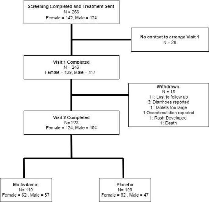
The hydration and dehydration protocol required a 12-h fast from food. The hydration protocol required subjects to drink water during the 12-h fast (at least 6, 8-ounce (237 mL) glasses for males and at least 4, 8-ounce (237 mL) glasses for females), while the dehydration protocol required a 12-h fast from fluid ingestion. Participants were reminded via email the day before their lab visit to begin the protocol exactly 12-h before coming to lab. Twelve hours was chosen to mimic the clinical relevance of fasting 12-h prior to common blood tests. For the control protocol, subjects maintained their normal dietary routine prior to measurements. Subjects reported to lab the same time of day for all protocols to control for diurnal rhythm. Each subject was required to complete all three testing protocols within a period of 7days to minimize effects from weight changes, with a washout period of at least 24 h between protocols. Of the 47 subjects, 1 did not follow the protocol on their hydration day and 5 had issues with blood draw. Data from these 6 subjects were removed from analysis leaving a total of 41 subjects who completed the study (Fig. 1).

Schematic representation of data collection from initial recruitment to data used for statistical analysis.

To determine hydration status, the following measurements were analyzed: spot urine osmolality (UOSM), spot urine specific gravity (USG), spot urine color (UC), body mass (BM), percent total body water (%TBW), hematocrit (Hct), hemoglobin concentration ([Hb]), plasma osmolality (POSM), serum osmolality (SOSM), plasma volume (PV), plasma volume status (PVS), and serum volume (SV). When a subject came to the laboratory, blood was drawn from a prominent vein in the antecubital space while seated [28] using a 21-gauge butterfly needle with a 7-inch luer lock extension connected to a vacutainer adapter (Becton-Dickinson, Franklin Lakes, NJ USA). Blood was collected into a 4 ml heparin and a 4 ml serum separation vacutainer (Becton-Dickinson, Franklin Lakes, NJ USA).

After blood collection, the subject entered a private restroom where he/she provided a urine sample, emptied his/her bladder completely, and then performed a naked body weight and %TBW measurement using the Tanita BC-533 bioelectrical impedance (BIA) scale (Tanita Corporation of America, Inc., Arlington Heights, IL USA). This scale was used due to its ability to give repeatable weight and %TBW measurements, as tested in-house prior to commencement of the study. This type of scale does not distinguish between intracellular water and extracellular water. The urine sample was not a first morning sample as first morning urine may not strongly correlate with fluid intake [29].

The urine sample was visually analyzed for color using the sample-over-chart method [30] in ambient fluorescent laboratory lighting by the same non-blinded investigator [31]. Urine Osmolality was measured using a single sample osmometer (Advanced Instruments Model 3250, Norwood, MA USA). Specific gravity was measured using an analog handheld refractometer (ATAGO U.S.A., Inc., Bellevue, WA USA).

Blood from the heparin vacutainer was used to determine Hct in duplicate (1.32% intra-assay coefficient of variation) by filling two microhematocrit tubes with blood from the heparinized vacutainer, which were then centrifuged at 13,700 × g for two minutes using a microhematocrit centrifuge (StatSpin CritSpin, HemoCue America, Brea, CA USA). Hematocrit was determined by measuring the height of blood and plasma divided by the height of red blood cells (RBCs) and multiplied by 100. A 10-fold dilution was performed by placing 1 ml of blood from the heparinized vacutainer into 9 ml of deionized water (dH2O) for 30 min to allow lysing of RBCs. Following this incubation period a 10-fold series dilution was performed two more times using dH2O to obtain a final 1000-fold dilution. This 1000-fold dilution was used to determine [Hb] via the Harboe method with an Allen correction factor [32]. Briefly, the 1000-fold diluted sample was poured into a cuvette and underwent spectrophotometry at the wavelengths of 380, 415, and 450 nanometers (nm) using an Eon spectrophotometer (BioTek Instruments, Inc., Winooski, VT USA). The absorbance at each wavelength, after subtraction from a dH2O blank, were used to determine [Hb] with a modified version of the Harboe equation to give hemoglobin results in g/dl instead of mg/dl. Thus, the following equation was used: Hb (g/dl) = ((0.01672 x A415) – (0.00836 x A380) – (0.00836 x A450)) * 1,000; where 0.01672 and 0.00836 are constants, A415 represents absorbance at 415 nm, A380 represents absorbance at 380 nm, A450 represents absorbance at 450 nm, and multiplying by 1,000 accounts for the 1,000-fold dilution.

Hematocrit and [Hb] were then used to determine plasma volume using the following equations developed by Dill and Costill, 1974 [7]:

$$}}_}}=}}_}}(}}_}}/}}_}})$$

where BV = blood volume, Hb = hemoglobin, CV = red blood cell volume, Hct = hematocrit, PV = Plasma Volume, A = after dehydration, B = before dehydration, BVB was considered to be 100.

Plasma volume was calculated with control values for [Hb] and Hct entered in the “before” part of the formulas and [Hb] and Hct values for dehydration or hydration put in the “after” part of the formulas to provide consistency of the PV calculations.

Plasma volume status has also been shown to be an accurate measure to assess plasma volume [33, 34]. Therefore, PVS was calculated according to Hoshika et al. [33]:

$$}\; }=(1-})* \left[}+(}}* }\; }\; }\; })\right.$$

$$}\; }=}}*}\; }\; }\; }$$

$$}( \% )=}\; }-}\; })/}\; }]}*100;$$

where PV = plasma volume, a = 1530 in males and 864 in females, b = 41 in males and 47.9 in females, kg = kilograms, c = 39 in males and 40 in females, PVS = plasma volume status.

The remaining 3 mL of blood in the heparin vacutainer underwent centrifugation at 2630 × g for 10 min at 4 °C (ThermoScientific Sorvall Legend RT+ refrigerated centrifuge, Thermo Fisher Scientific, Inc., Walthum, MA USA) to separate the plasma. Following centrifugation, POSM was determined via the single-sample osmometer.

3 mL of blood were removed from the serum separation vacutainer and placed into a serum transfer tube. This was done to ensure the same amount of blood was used to determine SV for each sample, as no formula exists for calculating SV. The 3 mL of blood was then allowed to coagulate at room temperature for greater than 30 min, but no longer than 60 min. Following coagulation, the blood underwent centrifugation at 2630 × g for 10 min at 4 °C. The separated serum was then poured into a graduated cylinder standing on a chemical scale (Mettler Toledo XS104, Mettler-Toledo, LLC, Columbus, OH USA) to determine SV produced per 3 mL of blood both by visual measurement using the graduated cylinder and by weighing the serum sample with the assumption that 1 µl of serum has a mass of 1 mg. Once the measurement of SV was complete, SOSM was measured via freezing point depression using the single sample osmometer. All measurements were performed immediately following blood and urine collection to avoid any fluid changes due to storage [35].

One subject forgot to measure %TBW on their control day creating one missing data point. To account for this, a multiple imputation approach using 5 imputations and taking the mean was used. The original data set of %TBW was then compared to the %TBW data following multiple imputation using a two-tailed paired T-test. Outliers for all variables were identified using the Z score method with cutoff points of 3.0 and −3.0. This decision was made a priori in order to remove subjects who likely did not comply with one of the protocols.

A repeated measures analysis of variance (RMANOVA) was used to compare all variables when multivariate normality was met. When Mauchley’s test of sphericity was not met, a Greenhouse–Geisser Correction factor was used. For variables in which multivariate normality was not met, a two-way Friedman’s non-parametric test was used. Bonferroni post-hoc analyses were used when significance was found to determine differences among variables. Partial eta squared (η2) was used to calculate effect size when RMANOVA was used, and Kendall’s W was used for a Friedman test.

To determine sex differences between age, a two-tailed independent samples T-test was conducted when the assumption of normality and homogeneity of variance for mean was met. A two-tailed Mann–Whitney U test was conducted when normality or homogeneity of variance for mean was not met. Cohen’s D (d) was used to calculate effect size when a two-tailed independent samples T-test was conducted and η2 was used to calculate effect size when a Mann–Whitney U test was conducted.

Sex differences for all other variables were compared using a multivariate ANOVA (MANOVA) with Pillai’s trace even if normality was violated, as long as homogeneity of variance was met, as the MANOVA has been found to outperform the nonparametric test when only the assumption of normal distribution is violated [36]. If the assumption of homogeneity of variance was violated, a nonparametric multivariate Kruskal–Wallis test was used.

Normality was tested using a Shapiro–Wilk Normality test. Homogeneity of variance was tested using a Levene statistic. Alpha was set at 0.05 to determine statistical significance. All statistical analyses were generated using the Statistical Package for the Social Sciences (SPSS) version 28 (SPSS Inc., Chicago, IL USA).