Patient selection

The study was approved by the local Institutional Review Board. The need for informed written consent was waived. The primary starting group of cases was collected from September 2022 to June 2024, with two qualifying characteristics establishing inclusion: (1) a high 2D planar LSF (≥ 8%), and (2) at least one CT with full lung coverage to establish a best estimate of full lung mass. All cases involved Theraspheres™ 90Y glass microspheres.

Lung mass estimate: MAA-CTs, 90Y-CTs, and diagnostic CTs

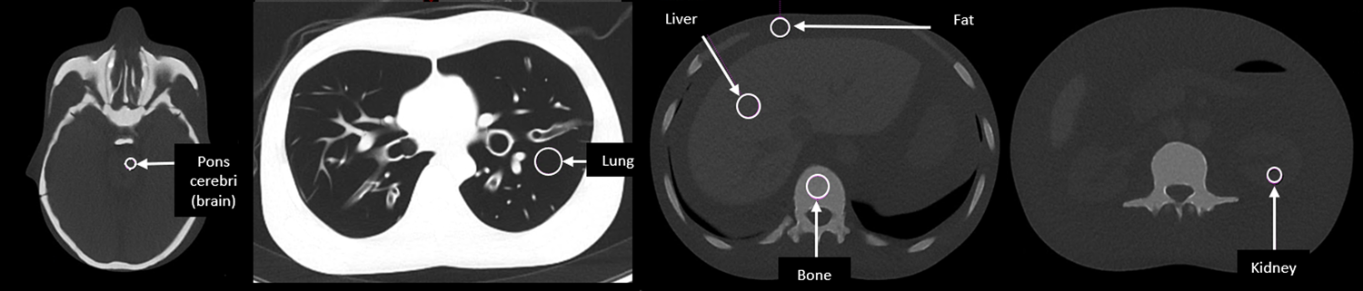
In order to establish a best estimate of full lung mass, MAA-CTs, 90Y-CTs, or diagnostic CTs covering the chest were searched and collected amongst the patients in the cases assembled. No restrictions were applied for collecting other CT datasets related to the use of iodinated contrast or time interval between longitudinal CT scans of each patient. CT scans from outside institutions were also allowed. For patients where multiple CTs with full lung coverage were available, the primary choice was the MAA-CT associated with the case at hand. The secondary choice was the CT closest in time to the MAA planning procedure. All CT datasets were used to define lung and liver volumes via auto-segmentation (Contour Protégé AI, MIM, Inc. v7.1.5). The lung and liver segmentations were reviewed and refined as necessary by a medical physicist (MAT) and then approved by at least one clinician. Lung mass was estimated using the previously outlined method involving lung mean Hounsfield unit (HU) value [8, 14]:

$$Lung\, Mass \left(g\right)=Lung\, Volume \left(^\right)\times \frac\times 1.04g/^$$

(1)

Cases were separated into groups on the basis of lung coverage in the MAA-SPECT/CT field of view. If the MAA-SPECT/CT maintained 100% coverage of the lungs, no other CT was needed. For cases with MAA-SPECT/CT lung truncation, lung coverage was estimated by comparing the MAA-CT lung mass to the estimated lung mass from a secondary CT. Due to the possibility of the SPECT and CT acquisitions maintaining different coverages of the lungs, the lung coverage was determined by the SPECT rather than the CT. As an example, a case may have shown 100% lung coverage in the CT but < 100% in the SPECT. CT contours of the lungs were adjusted to reflect the limits of coverage in the SPECT. Cases were categorized into two groups based on this strategy: (1) FOV ≥ 90%, where MAA-SPECT/CT lung coverage was complete or nearly complete (≥ 90%), and (2) FOV < 90% where lung coverage was < 90%.

Planar and MAA-SPECT/CT acquisition and reconstruction

Planar and MAA-SPECT/CT scans were acquired on one of four SPECT/CT scanners (Siemens Symbia T6, GE Optima 640, GE Optima 670, or GE 870). All scanners used low energy high resolution (LEHR) collimation except for the GE 870 which used LEHR Sensitivity. A photopeak window centered at 140 keV was used for all scanners, with 15% (Siemens) and 20% (GE) window widths, and 18% (Siemens) and 10% (GE) scatter windows. All planar acquisitions were two beds, one centered over the lungs and one centered over the liver (abdomen), at 5 min each. All SPECT/CT scans used a single bed position focused on encompassing the entire liver and relevant areas of the abdomen as opposed to ensuring full lung coverage. The scans were for 120 views over 360° at 15 s/view except for the GE 870 at 20 s/view, and all scans implemented auto-contouring. MAA-SPECT reconstruction was ordered-subset expectation maximization with a 128 × 128 matrix for all scanners, with 4 iterations and 10 subsets for GE and 8 iterations and 4 subsets for Siemens. Siemens reconstructions included a 8.4 mm Gaussian filter while GE used a 8.0 mm Gaussian filter as well as Resolution Recovery. The CT acquisitions in the MAA-CTs varied by scanner, but used 120 or 130 kV, a pitch from 0.8 to 1.4, 10–20 mm collimation, 0.8–1.0 s rotation time, 90–150 mA tube current, and a computed tomography dose index volume (CTDIvol) of 8–10 mGy. The GE Optima 640 used a much lower CTDIvol of ~ 3 mGy (30 mA). CT images were reconstructed using soft tissue kernels (GE: STD, Siemens: B31s) and no iterative reconstruction. SPECT voxel sizes were 4.4 × 4.4 × 4.4 mm (all GE) or 4.8 × 4.8 × 4.8 mm (Siemens), while CT voxels were 1 × 1 × 5 mm (GE 670 and 870), 1 × 1 × 2.5 mm (GE 640), or 1 × 1 × 4 mm (Siemens).

LSF and LMD calculations

LSF was calculated using Eq. (2) below, with different methods utilized to determine lung and liver counts.

$$LSF= \frac_}_+ _}$$

(2)

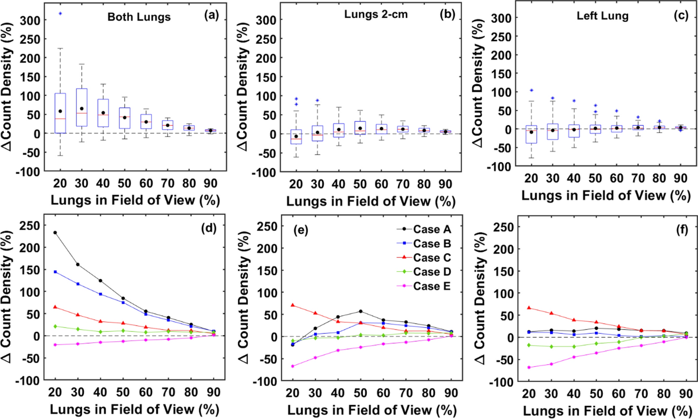
For planar LSF, the geometric mean of anterior and posterior views from the 2D planar images was used for determining counts [8]. For the SPECT/CT methods, counts were computed from SPECT using the lung and liver contours defined on the CT from the relevant MAA-SPECT/CT. In some cases, a rigid registration was applied to the SPECT to correct for misregistration with the CT near the diaphragm. This was to avoid biasing the assignment of counts between the liver and lungs in cases with clear misregistration. Three different sets of liver and lung segmentations were used for establishing counts in the SPECT/CT methods. (1) Both Lungs: the liver and lung contours were used directly without any adjustments or corrections. (2) Lungs 2-cm: the liver contour was expanded by 2 cm in all directions, and this contour was used to determine liver counts. Any intersection of the expanded liver contour with the lungs was removed, then the adjusted lungs contour was used to determine a lung count density (counts/g). The lung count density was then applied to the full lungs mass to establish the corrected lung counts value [8, 11, 13]. (3) Left Lung: any intersection of the expanded liver contour with the left lung was removed, then only the left lung was used to determine a lung count density and corrected lung counts were calculated as with 2) above. The 2-cm expanded liver contour was again used for liver counts. For all three strategies to categorize counts to the liver and lungs, no counts were dually assigned to both regions. LMD was calculated using Eq. (3) below:

$$LMD (Gy)= \frac\right)\times AA(GBq)\times LSF}$$

(3)

Truncated lung conditions: theoretical impacts on LSF and LMD

If uniform count densities (counts/g) are assumed, LSF and LMD estimates can be calculated by extrapolating the data at < 100% lung coverage all the way to full lung coverage. The relationships between the estimated LSF and LMD at limited field of view (LSFTrunc, LMDTrunc) and the uniformly extrapolated LSF and LMD at 100% lung coverage (LSFUniform, LMDUniform) can be determined. A detailed outline of this analysis is included in the Supplemental Information. The key relationships that compare truncated and uniformly extrapolated LSF and LMD are as follows:

$$_Uniform\\ ratio\end}=\frac_}_}=_+_\times (1-_)$$

(4)

$$_Uniform\\ ratio\end}=\frac_}_}=\frac_Uniform\\ ratio\end}}_}$$

(5)

In Eqs. (4,5), \(_\) is the fraction of lungs (by mass) in the truncated FOV, and the LSF and LMD ratios outlined provide a sense of the error related to computing LSF and LMD under truncated conditions. Using these equations, simulated errors in LSF and LMD were computed across a range of lung truncation levels using three different values for LSFTrunc to represent low, medium, and high clinical LSF values (2.5, 7.5, and 15%).

Lung count density variations and modeling

The equations outlined in the previous section apply only to assumptions tied to uniform count density throughout the entire lung volume. For cases with non-uniform count densities, LSF and LMD estimates based on a uniform extrapolation of truncated MAA-SPECT/CT data may lead to significant errors. Variations in lung count density were analyzed by computing lung counts/g at different simulated levels of lung truncation, and then calculating the changes in lung count density relative to full lung coverage. To collect this data, the lung segmentations from the FOV ≥ 90% cases were modified by removing axial slices starting at the most superior slice and continuing inferior toward the diaphragm in ~ 5 mm increments. A wide range of lung coverages from 100% to < 1% in ~ 2% increments were created for Both Lungs, Lungs 2-cm, and Left Lung. Lung counts, mean lung HU (lung mass), and lung volume were collected for all the adjusted contours.

Different empirical models were considered to fit the variations in lung count density for the cases in the FOV ≥ 90% group. Two simple model types were explored:

$$Power\, Function: Lung\, Counts=A\cdot _)}^$$

(6)

$$Linear\, Function: Lung\, Counts=C\cdot _+D$$

(7)

Lung counts were modeled using lung mass as the input variable, masslung. Model fits were determined for simulated lung fractions from 20 to 90%. Lung counts at full lung mass were predicted from the empirical fits and then used in LSF and LMD estimates. Note that a generalized model was not developed using all cases. Rather, each case was independently fit using its unique lung mass and lung counts data. A main objective of the case-by-case empirical fits was to better understand the non-uniformities in count density for each case, and then use the results of the model fits to strategize corrections for LSF and LMD estimates. More details about the fitting process and information about how the fitting parameters were used to predict lung counts are included in the Supplemental Information.

LSF and LMD estimation methods and errors

Different types of LSF and/or LMD estimates were calculated using different versions of lung counts and/or lung mass. The methods are named and described below. For methods (1), (3), and (4), lung mass was the full lung mass from the MAA-CT.

1.

Planar: LSF and LMD calculated using Eqs. (2) and (3), lung counts and liver counts computed from 2D planar imaging; note that the lung mass used here is different from the recommendation in the vendor IFUs, where a standard reference mass of 1-kg is used

2.

SPECTTrunc: LSF and LMD calculated using Eqs. (2) and (3), with the lung counts and lung mass computed from only the MAA-SPECT/CT data available at truncated lung coverage (no extrapolations or corrections applied)

3.

SPECTUniform: LSF and LMD calculated using Eqs. (2) and (3), with lung counts computed from a uniform extrapolation of the lung count density at truncated lung coverage up to the full lung mass

4.

SPECTFit: LSF and LMD calculated using Eqs. (2) and (3), with lung counts predicted at the full lung mass from the case-specific empirical model fit [Eqs. (6,7)].

Percent errors were also calculated between the various LSF and LMD estimates and ground truth. Detailed analysis of errors and the various correction methods was applied to simulated lung coverages of 40, 60, and 80% to best represent significant, average, and minimal lung truncation as observed in clinical cases.

Lung mass estimate errors: impact on LSF/LMD calculations

Several aspects of the proposed workflow and strategies for LSF and LMD corrections outlined in this work require a best estimate of full lung mass. Once a CT with full lung coverage is identified, there may still be concern that the lung mass estimate derived from that CT maintains bias or uncertainty. We therefore assessed the impact of lung mass uncertainty on the various calculation and correction methods proposed in this work. The details of this analysis are provided in the Supplemental Information. The relationships between lung mass error and LSF or LMD error were derived for both uniform and non-linear correction methods for lung counts. Assumed lung mass errors from − 50 to + 50% were applied to the derived LSF and LMD error equations to establish the impact of lung mass errors across the different correction methods analyzed.

Application of estimation methods to FOV < 90% cases

To showcase the utility of LSF and LMD corrections under truncated lung conditions, the methods described herein were applied to the FOV < 90% group of cases. LSF and LMD values using planar, SPECTTrunc, SPECTUniform, and SPECTFit were computed and compared. The estimated full lung mass (from a different CT) that determined the level of lung truncation was used in all LSF and LMD calculations. The full details of how the SPECTFit method was applied to the cases from the FOV < 90% group can be found in the Supplemental Information. To explore the impact of each estimation method on the corrections, the coefficient of variation (COV) between the LSF and LMD values as estimated by SPECTTrunc, SPECTUniform, and SPECTFit was computed. COV values were then correlated to the level of lung truncation in the clinical cases to better understand its effect on the variation in estimates from each method.

Statistical analysis

Datasets analyzed in this work were first tested with both Anderson–Darling and Shapiro–Wilk normality tests. Datasets were determined to be both normally and non-normally distributed. As a result, both parametric and non-parametric significance tests were used as appropriate. Mean ± σ was used for comparisons. For all matched comparisons among paired datasets, repeated measures one-way ANOVA analysis was used for normally distributed data while Friedman’s tests were used in other cases. If a statistically significant difference among all groups was established, multiple comparisons were assessed for more specific analysis among groups. A false discovery rate correction using the two-state step-up method of Benjamini et al. [15] was also implemented using a false discovery rate of 0.05, with all p values reported after adjustment for multiplicity. All statistical analyses were performed with GraphPad Prism 10.3.1 (GraphPad Software, San Diego, California, USA) and statistical significance was considered true for p < 0.05. In order to better understand the different LSF and LMD calculation methods, mean differences and 95% prediction intervals (± 1.96σ, PI) of differences between calculation methods were computed as outlined in Bland–Altman analysis [16, 17]. Limits of agreement (LoA) were determined as mean ± 95% PI.