Study population

The study cohort consists of 110 DTC patients (74 females and 36 males) aged between 14 and 85 years who underwent postoperative RAI therapy between September 2018 and February 2023 in Turku University Hospital, Finland. Two patients who received RAI during this period, while remote DRMs were in maintenance, were excluded. According to the clinical practice all patients had previously undergone total thyroidectomy.

Pathology and laboratory tests

Histological status of cancer was determined from pathologic-anatomical diagnosis (PAD) along with the presence of possible lymph node metastasis in the sample. Additionally, the tumor characteristics were also investigated. TNM-staging was done for the majority of patients based on AJCC/UICC staging system [15]. Patients were referred to RAI ablation based on the stage classification and medical eligibility according to clinical practice. The medical history of the patients were also reviewed.

Laboratory tests including thyroid-stimulating hormone (TSH), thyroglobulin (TG), serum creatinine (sCr), and glomerular filtration rate (GFR) were done prior ablation.

Patient preparation and RAI therapy

Patients adhered to a low-iodine diet for two weeks. Due to the coronavirus outbreak in 2020, the iodine-deficient diet for two patients was shortened by a few days. TSH stimulation (> 30 mU/l) was achieved with two thyrotropin alpha (Thyrogen®) injections, administered 24 and 48 h before the RAI treatment. TSH and serum TG were monitored the same morning before to ensure successful TSH stimulation level for the ablation and TG for a reference value for patient follow-up.

Patients were given oral and written information regarding the progress of RAI treatment in the department and radiation protection during hospitalization and after discharge from the hospital. In Finland, standardized activities of 1.11 GBq and 3.70 GBq were employed, according to the cancer characteristics and the risk of its recurrence [16, 17]. For subsequent treatments, a 3.70 GBq activity of RAI was employed.

All patients were hospitalized in one of our two radiation-protected isolation rooms typically from 1 to 3 days [6, 16]. The patients were discharged from the hospital when their external dose-rate was less than 15 µSv/h measured at a distance of one meter with a hand-held DRM [8]. The patient may also be discharged, if the measured dose-rate is between 15 and 40 µSv/h at the discretion of medical physicist, along with individual tightened radiation protection instructions. The discharge limit was chosen to fulfil national dose limits for family members and individuals [18].

Cloud-based remote dose-rate meters

The whole-body Teff of patient was determined by measuring the external dose-rate acquired with one of the two remote cloud-based DRMs (Sensire Dosimeter, Sensire, Finland) containing KATA DGM-1500 Turva DRM (KATA, Finland) that utilizes an ambient dose equivalent-energy compensated Geiger-Müller counter [19]. DRMs were installed in the ceilings of both isolation rooms, located approximately two meters above the hospital bed, continuously monitoring the dose-rate of their surroundings.

The data were collected at one-minute intervals, enabling the system to generate a nearly real-time graph of dose-rates as a function of time. To achieve individual patient records, the data were meticulously downloaded into separate .xlsx-files for each patient.

Dose-rate meter calibrations

The measured dose-rate signals are affected by patient’s movements in the room during isolation as well as radiation attenuation by the body. To ensure more accurate readings, patients’ location and position changes were incorporated using correction factors (CFs) obtained through calibration with a moderate-activity (A = 485 MBq) point source, a 131I capsule. Remote DRMs have a reasonable linearity (± 10.0%) over a wide range of dose-rates (0.01–100,000 µSv/h), which allows the use of a less-radiation-toxic source for calibration.

Calibration measurements were executed at three different locations in both rooms, where patients were most likely to spend time during isolation, such as laying supine or sitting on the patient bed and sitting on a chair by a table (approx. 2.0 m, 2.1 m and 3.5 m from the remote DRM, respectively). Laser distance meter (Fluke 424D, Fluke Finland Oy, Finland) was utilized to determine the distances between the DRM and these three measurement points. Five time-points average dose-rate values were measured at each location for the final calculations. The CFs were calculated as a ratio of the dose-rate reading measured in the supine position on the bed (reference location) to that measured in one of two other calibration locations. Additionally, the radiation attenuation by the body was compensated in the sitting position on the bed by estimating the path of radiation through the patient body and utilizing an attenuation coefficient specific to 131I in the water. The attenuation correction was carried out only in the single position because the attenuation effect was approximated to be the same in two other calibration locations. CFs made possible to correct fluctuations in dose-rate signals due to changes in the patient’s location and position in the isolation room.

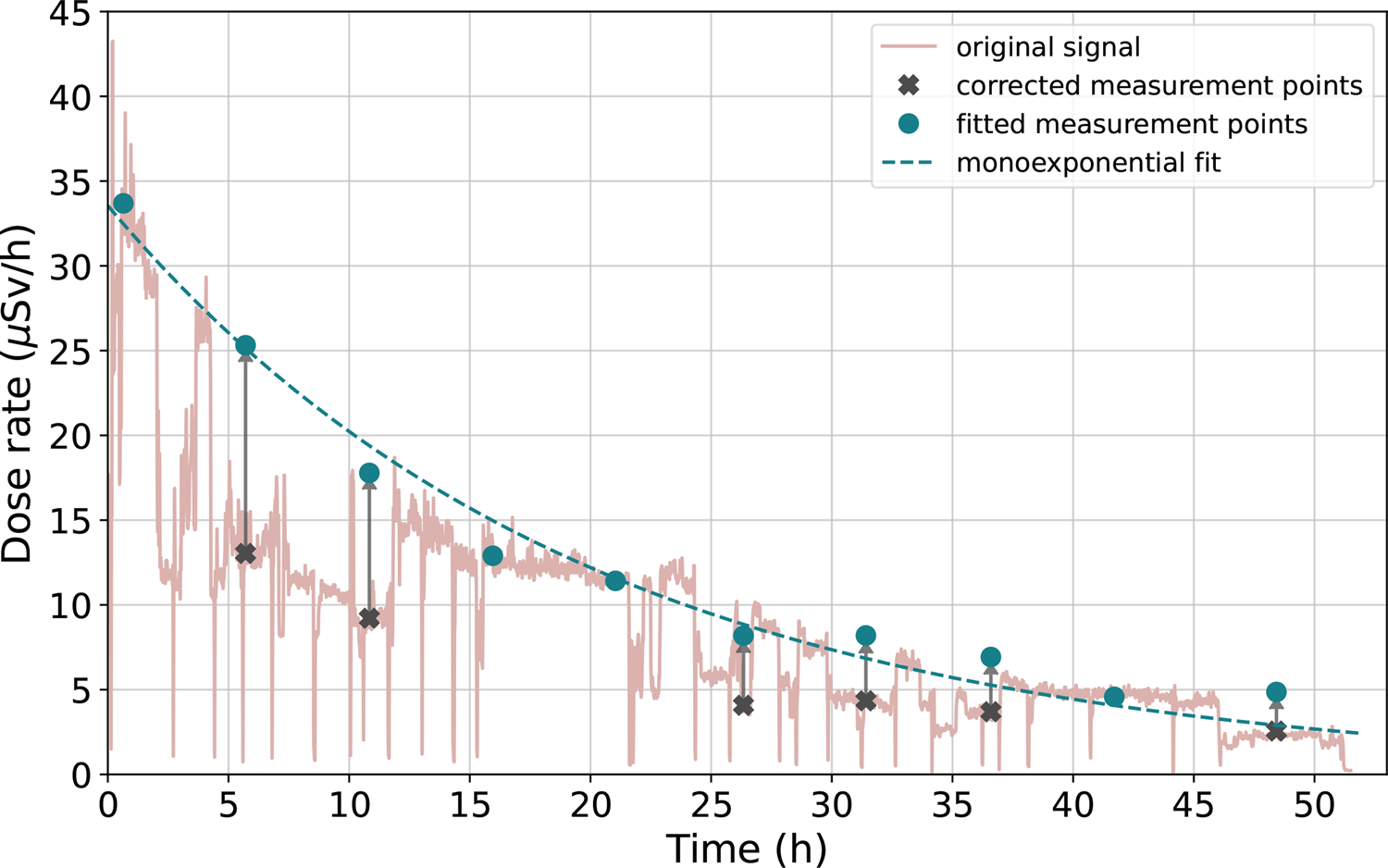
Preprocessing of measurement signals

To ascertain Teff of patients, ten measurement points were extracted from each patient’s dose-rate signal. The initial measurement point was selected within the first ten to thirty minutes after RAI administration. Subsequent measurement points were sampled evenly throughout the isolation period, from administration to discharge, providing a comprehensive representation of the clearance process. Due to the retrospective nature of our study, 13.8% of the sampled data points were corrected afterwards. Two CFs (1.97 for short distance and 2.10 for long distance) defined based on the calibration procedure described above were employed to adjust the dose-rate values. Background dose-rate was subtracted before curve fitting. Figure 1 visualizes the use of CFs in practice. To determine the Teff, a monoexponential function was fitted to the selected measurement points. The Teff was calculated from the fitted equation.

Fig. 1

An example remote dose-rate signal from 2.0 m distance during the isolation of a patient who received 3.70 GBq RAI. Original signal from the remote DRM is shown with light pink color. Before fitting a monoexponential function to measurement points (blue dots), some of the dose-rate values (black ticks) were corrected using the location CFs

Statistical analysis

The goodness of the monoexponential fits were evaluated by R-squared values (R2) that were calculated with Microsoft Excel 2016 v. 16.0 (Microsoft Office, Microsoft Corporation, USA). One-dimensional K-means clustering analysis was performed to identify similarities within the distribution of the Teff values. The clustering analysis was performed using Python v. 3.10 with three predefined clusters.

Logarithmical (Log) transformation was used to transform Teff data to conform normality. Normality assumptions were then evaluated visually using histograms and quantile-quantile (Q-Q) plot with standardized residuals of logarithmic values of Teff. Generalized linear mixed model (GLMM) was used to analyze the relationship between Log Teff and the original 26 patient characteristics. Parameters that were known to correlate with each other or were calculated based on another parameters, such as GFR and sCr, were excluded from the extensive GLMM analysis. The reduced GLMM model was constructed with parameters known to be significant based on the scientific literature and by removing one-by-one the least significant parameters based on the obtained p-values [9,10,11, 20,21,22,23,24,25,26]. The final GLMM model consisted of the seven most significant parameters: age, body mass index (BMI), GFR, other comorbidities, TG, administered activity, and treatment cycle. Statistical significance level was set at 0.05 and 95% confidence intervals (CI) were calculated. Categorical variables were described in percentage proportions and continuous variables which followed normal distribution with mean and standard deviation (SD) and otherwise with median and first and third quartiles (Q1, Q3). The analyses were carried out using IBM SPSS software package (v. 29.0 SPSS Inc., IBM Company, USA).