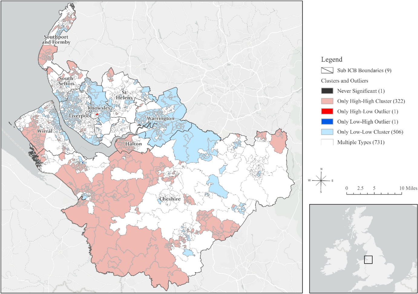
In this study, we focussed on the Cheshire and Merseyside Integrated Care System (ICS) in England, which consists of 1,562 Lower Super Output Areas (LSOAs) with an average population of 1500 people [12]. We used the LSOA boundaries published by the Office for National Statistics as of 21 March 2021 [12] and the digital vector boundaries for Integrated Care Boards, in England, as at April 2023 to compare sub-integrated care board locations in Cheshire and Merseyside ICS(Cheshire, Halton, Knowsley, Liverpool, South Sefton, Southport and Formby, St Helens, Warrington, Wirral).

We utilised the Combined Intelligence for Population Health Action (CIPHA) shared dataset, an individual-level, linked dataset established during the COVID-19 pandemic for continuously updated population health management [13]. Covering 97% of the registered population (~ 2.7 million people), this dataset includes demographic characteristics, primary care records, and LSOA-based residential information updated as patients notify general practitioners (GPs) of address changes. To estimate population sizes, we linked this dataset to the Office for National Statistics mortality register.

We then linked primary care records of all GP consultations from the beginning of year 2013 to the end of 2022 to estimate the prevalence and incidence of hearing loss over the past decade. We calculated hearing loss prevalence using Systematized Nomenclature of Medicine Clinical Terms (SNOMED) codes capturing all hearing loss types, from 2013 to 2022. For this study, we combined all available SNOMED codes on hearing loss to generate time series estimates of hearing loss prevalence for each LSOA over the study period.

A disclosure risk assessment was conducted following the ISB1523 Anonymisation Standard for Publishing Health and Social Care Data. To protect privacy, any numerators below five were suppressed if the denominator was ≤ 1,000 cases. The full list of codes and descriptions, including suppressed hearing loss types, is provided in Supplementary Material Table S1.

To account for differences in age structure across populations, we applied a rigorous age-adjustment process. The population was stratified into specific age groups (51–60, 61–70, 71–80, and 81 +), and hearing loss rates were calculated for each age group within each LSOA. These rates were then standardised using the age distribution of a standard population to derive a weighted average rate per LSOA and year. This adjustment was crucial to ensure that observed variations in hearing loss rates reflected true differences in prevalence rather than differences in the underlying population age composition.

Using age-adjusted prevalence estimates, we calculated the annual aggregate hearing loss diagnoses per LSOA by taking the weighted average count of the number of patients aged 50 years and older diagnosed with any type of hearing loss per LSOA and dividing it by the mid-year population estimates of individuals aged 50 and older within each LSOA. This approach ensured that the final rates accounted for both age structure differences and population size variations across areas and over time, enabling meaningful comparisons of hearing loss prevalence.

To provide additional context and test the spatial association with hearing loss prevalence, we incorporated the Index of Multiple Deprivation (IMD), a widely used measure of relative deprivation in the United Kingdom. We used the most recent English Index of Multiple Deprivation (IMD 2019), which provides detailed measures of deprivation across England [14] at high spatial resolution, or in small areas.

In a univariate analysis, the prevalence of hearing loss was described for each year using central tendency measures (mean and median) and dispersion measures (range, standard deviation, variance, minimum and maximum values). To assess spatial autocorrelation [15] across the region, we applied the Global Moran’s I statistic [16] for each year to measure spatial autocorrelation in values of hearing loss and to test whether the observed pattern was clustered, dispersed, or random.

Guided by the results of Global Moran’s I, we performed Cluster and Outlier Analysis, using the Anselin Local Moran’s I algorithm to identify local indicators of spatial association (LISA) and correct for spatial dependence [17]. The LISA identified statistically significant spatial clusters of small areas with high values (high/high clusters) and low values (low/low clusters) of hearing loss, as well as high and low spatial outliers—where a high value is surrounded by low values (high/low clusters) and vice versa (low/high clusters). Extending our spatial methods, we conducted a spatiotemporal analysis [18] of total hearing loss prevalence per LSOA for which there were no suppressed values; this analysis used an ecological space–time implementation of the Anselin Local Moran’s I statistic to identify statistically significant clusters and outliers in the context of both space and time [18].

We then created a set of three clusters based on the similarity of time series values. These clusters reflected approximately equal values across time, representing high, medium, and low rates of increase. Selecting three clusters was deemed optimal for supporting ongoing research examining the link between hearing loss and the three clusters of high, medium, and low rates of depression, as described in our recently published work [19].

To predict hearing loss trends from 2023 to 2027, we applied Curve Fit 5-year Forecast, assuming a continuation of trends observed from 2013 to 2022. Multiple forecasted space–time cubes were compared and merged to identify the best forecast for each location based on the Validation Root Mean Square Error (RMSE), assessing linear, parabolic, S-shaped (Gompertz), and exponential curve types. For the validation process, we used the Auto-Detect option for the Curve Type parameter, which fit all four curve types at each location and selected the one with the smallest Validation RMSE.

To understand the local effects of deprivation (IMD 2019) on hearing loss in 2020, we applied the Geographically Weighted Regression (GWR) model, which is suitable for spatial distributions exhibiting statistically significant non-stationarity [18, 20]. GWR is a local regression model that constructs a single equation for each feature in the study area using only its neighbouring features, allowing variable relationships to change across space. As a result, GWR produced the local R-squared values for each feature in the study area.

Statistical significance was set at the 99% confidence level to enhance the robustness and stringency of our results. Analyses were performed in ArcGIS Pro Version 2.9.2 [21] using the following tools, in order of execution: Spatial Join tool, Spatial Autocorrelation tool, Optimised Outlier Analysis tool (999 permutations), Space–Time Cube Creation tool, Space–Time Pattern Analysis tool, Evaluate Forecasts By Location tool, Time Series Clustering tool, and Tabulate Intersection tool.