False-negative rates from viral dynamics model

Critical to determining the effectiveness of border measures is the false-negative rate of viral tests, including PCR tests, which is influenced by the viral load and the ability of the test to detect the virus (detection limit). Since the viral load varies throughout the course of an infection, increasing initially, reaching a peak, and then declining, the false-negative rate also changes over time [16]. In a previous study, we estimated false-negative rates for PCR tests for SARS-CoV-2 using a mathematical model of within-host viral dynamics, considering the timing of tests and different detection limits [19]. Here, we adapted the same within-host modeling framework to estimate the false-negative rate of PCR tests for MPXV. Specifically, we reparameterized the model using MPXV viral load data from relevant anatomical sites (rectum, saliva, and oropharynx). Although the transmission dynamics of SARS-CoV-2 and MPXV differ, our focus was on within-host viral kinetics, which allows this modeling framework to be transferable across infections with different transmission routes.

MPXV viral load data

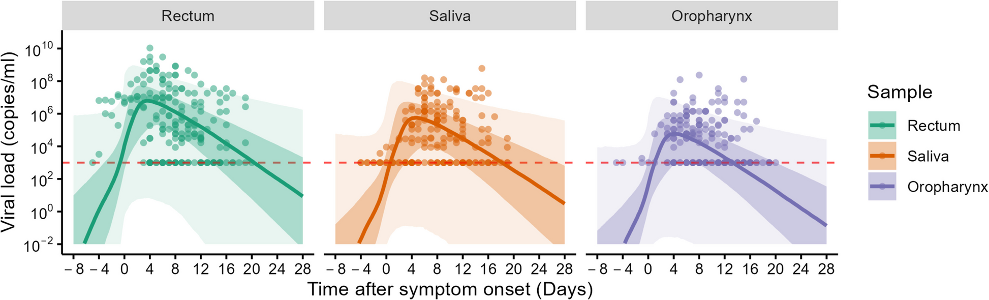
To parameterize the viral dynamics model, we analyzed two prospective longitudinal cohort studies. The first cohort enrolled 77 men with acute mpox infections (clade IIb) hospitalized in Shenzhen, China, between June 9 and November 5, 2023 [20]. Participants were followed up to 21 days after symptom onset. Samples were collected every 2–3 days from various sites, including skin lesions, rectum, saliva, oropharynx, urine, and plasma. The second cohort enrolled 25 individuals who had high-risk contact with mpox-infected patients in Antwerp, Belgium, between June 24 and July 31, 2022 [21]. Participants were followed up for a maximum of 21 ± 2 days after inclusion, while infected participants were monitored until they tested MPXV-PCR positive with typical mpox symptom onset and then referred to routine clinical care. During weekly follow-up visits, blood, saliva, oropharyngeal swabs, genital swabs, anorectal swabs, and skin lesion swabs were collected. Additionally, anorectal swabs, genital swabs, and saliva were also collected through daily self-sampling. PCR sensitivity was higher with oropharynx, saliva, rectum, and skin lesions (> 70%), while PCR sensitivity was lower with urine, serum, genital swabs, and plasma samples (< 50%). Hence, we have focused our analysis on samples with higher PCR sensitivity (oropharynx, saliva, and rectum) for ITC purposes. It is worth noting that we have excluded the skin lesion data in the analysis, as PCR testing on skin lesions can only be conducted after lesions are visible. Therefore, relying on skin lesions for PCR testing at immigration to identify infected individuals is moot. Both cohorts included individuals infected with MPXV clade IIb, which caused the 2022–2023 global outbreak. No data from clade I or clade Ia infections were available for model fitting. Quantitative real-time PCR (qPCR) was used to measure cycle threshold (Ct) values. To convert the Ct value to viral load, we applied the following equation: \(\text=-3.611(}_\text)+41.388\) as described in the paper [20]. Ct values > 40 (i.e., < 103 copies/mL for viral load) are considered negative.

Viral dynamics model and fitting

To characterize the MPVX viral dynamics, we used the following system of ordinary differential equations, which accounts for the fundamental biological process of the infection within a host, including viral replication and elimination due to immune response:

$$\frac=-\overbrace^\;\mathrm\;\mathrm\;\mathrm},$$

$$\frac=\stackrel}}-\stackrel}},$$

$$\frac=\overbrace^\text-\overbrace^\text,$$

where the variables \(T(t)\), \(I(t)\), and \(V(t)\) represent the number of uninfected target cells, number of infected target cells, and amount of virus at \(t\) days after symptom onset, respectively. These represent the infection of uninfected cells at rate \(\beta T\left(t\right)V\left(t\right)\) and the removal of infected cells at rate \(\delta I\left(t\right)\) cells per day, and the production of virus at rate \(pI\left(t\right)\) and the removal of virus at rate \(cV\left(t\right)\) viral units per day. Note that we use days after symptom onset as the time scale. The model parameters \(\beta\), \(\delta\), \(p\), and \(c\) represent the rate of virus infection, death rate of infected cells, (per cell) viral production rate, and (per capita) clearance rate of the virus, respectively. Under the quasi-steady-state assumption, the model is reduced to a two-dimensional model as follows:

$$\frac=-\beta g\left(t\right)V\left(t\right),$$

$$\frac=\gamma g\left(t\right)V\left(t\right)-\delta V\left(t\right),$$

where \(g(t)\) is the fraction of uninfected target cell population at day \(t\) to that at day 0 (i.e., \(g\left(0\right)=1\)), and \(V\left(t\right)\) is the amount of virus at day \(t\) (copies/mL), respectively. Note that time 0 corresponds to the day of symptom onset. Details on the transformation of this model are reported in the reference [22]. The quasi-steady-state assumption is generally reasonable for most viruses causing acute infectious disease because the clearance rate of virus (\(c\)) is typically much larger than the death rate of the infected cells (\(\delta\)) as evidenced by in vivo observations [22,23,24]. Thus, we estimated the four parameters: \(\beta\), \(\gamma\), \(\delta\), and \(V\left(0\right)\) (viral load at the day of symptom onset). We fit the viral dynamics model to the viral load data collected from the three different sites (rectum, saliva, and oropharynx) independently using a nonlinear mixed effect model.

The nonlinear mixed-effects model incorporates fixed effects and random effects accounting for inter-site variability in viral dynamics. Specifically, the parameter for site \(k\), \(_\left(=\theta \times ^_}\right),\) is represented by the fixed effect, \(\theta ,\) and the random effect, \(_,\) is assumed to follow the Gaussian distribution with mean \(0\) and standard deviation \(\Omega\). The fixed effect (population parameter) and random effect were estimated by using the stochastic approximation expectation–maximization (EM) algorithm and empirical Bayes’ method, respectively. We chose these methods because the EM algorithm is well-suited for estimating population-level parameters in the presence of latent variables, whereas the empirical Bayes allows us to efficiently estimate inter-site-level variations by using prior information. Using estimated parameters and a Markov Chain Monte Carlo (MCMC) algorithm, we obtained the conditional distribution of model parameters for each site. Left censoring was considered based on the lower limit of detection (Ct values < 40). Monolix 2023R1 (https://www.lixoft.com) was used for viral dynamics model fitting.

Simulation analysis to estimate false-negative rates over time

We repeatedly randomly resampled a parameter set for individual \(i\) at site \(k\) (i.e., \(_\), \(_\), \(_\), and \(_\)) from the estimated posterior distributions, and ran the viral dynamics model. The viral load obtained by running the viral dynamics model is considered as the “true” viral load, \(_(t)\). However, PCR test results are influenced by measurement error. To account for this, we added measurement error to the true viral load to simulate measured viral load, \(}_(t)\), whereby \(}_}_(t)=}__(t)+_\), \(_\sim N\left(0,_^\right)\) [25, 26]. As the time scale of the viral dynamics model is days after symptom onset, we corrected the time scale to time after infection by adding incubation period, \(\eta\), drawn from the incubation period distribution obtained from the meta-analysis [10]. That says, \(_\left(\tau \right)=_\left(t+\eta \right)\), \(\eta \sim \textN(\text)\) (mean = 8.1, 95th percentile = 18), where \(\tau\) is the infection age (i.e., the time which has elapsed since infection). The error distribution is obtained by fitting a normal distribution to the residuals (i.e., the difference between the common logarithms of the true viral load and the measured viral load). We repeated this process 10,000 times to create the viral-load distribution over time. The false-negative rate at site \(k\) at infection age \(\tau\) is computed as the proportion of cases with a viral load below the detection limit: \(_(\tau )=_^I(}_(\tau )<DL)/1000\), where \(DL\) is the detection limit, and \(I\) is the identity function. We used 250 copies/mL as the detection limit of PCR tests [27]. As a sensitivity analysis, we performed the same simulation using different detection limits, namely 10 and 1000 copies/mL.

Detection rates by health screening and PCR tests and post-entry incubation periods for travelers

To assess the impact of health screenings and PCR tests, we examined a population of individuals infected during travel in mpox-affected countries and moving to non-mpox-affected countries. In this study, we define “mpox-affected countries” as those actively reporting mpox cases during the simulated period, regardless of whether they were historically endemic (i.e., prior to 2022) or only recently affected. Note that the infected traveler population in our analysis represents a hypothetical population. Specifically, we simulated infection age distributions based on assumed epidemic growth rates in the countries of origin and assigned viral load trajectories estimated from the two cohorts to our simulated travelers. Upon arrival in non-mpox-affected countries, the time elapsed since infection, referred to as the infection age (\(\tau\)), represents the duration between the date of infection and the date of arrival at the travel destination. Assuming that mpox cases in the country of origin are either exponentially increasing (growth rate, \(r>0\)) or stable (endemic, \(r=0\)), and that travelers are exposed proportionally to the number of cases, the number of infected (traveling) individuals with infection age \(\tau\) at immigration is described as follows: \(j\left(\tau \right)=_\text(-r\tau )\), where \(_\) is a constant number representing those at infection age \(\tau =0\) (\(j\left(0\right)=_\)). Given that health screenings at immigration detect individuals with symptoms, we aim to use PCR tests to identify asymptomatic individuals at the time of entry. These individuals are modeled as being in the early stages of infection, where the infection age \(\tau\) is below the threshold for symptom manifestation. The number of pre-symptomatic individual with infection age \(\tau\) at immigration, modeled as \(_\left(\tau \right)=_\text(-r\tau )L\left(\tau \right)\), where \(L\left(\tau \right)\) is the survival function of symptom development by infection age \(\tau\). The survival function of symptom development \(L\left(\tau \right)\) can be computed from the probability density function of incubation period, \(f\left(\tau \right)\), as \(L\left(\tau \right)=1-_^f(u)du\). The number of pre-symptomatic individuals who test negative for mpox on PCR tests conducted at immigration is represented by \(_\left(\tau \right)=_\text(-r\tau )L\left(\tau \right)p(\tau )\), where \(p\left(\tau \right)\) is the false-negative rate of PCR tests at infection age \(\tau\). The proportion of infected travelers who develop symptoms and are subsequently identified by the health screenings at immigration (including those who canceled travel due to symptoms) can be modeled as \(H=1-\frac_^_\left(u\right)du}_^j\left(u\right)du}=1-\frac_^\text(-ru)L\left(u\right)du}_^\text(-ru)du}\). This assumes that the health screenings detect all symptomatic mpox cases. The proportion of infected travelers identified through PCR testing can be modeled as \(T=\frac_^_\left(u\right)-_\left(u\right)du}_^j\left(u\right)du}=\frac_^\text\left(-ru\right)L\left(u\right)(1-p\left(u\right))du}_^\text(-ru)du}\). Note that \(_\) is canceled in the derivation process of \(H\) and \(T\).

The quarantine period can be determined based on the incubation period, assuming that the time of exposure is known—typically the 95th percentile of the incubation period distribution [28]. However, in this study, we assume that the timing of exposure is not known and only the timing of entrance to the country is known. Therefore, the quarantine period begins upon entry into the country. To determine the appropriate length, we estimated the remaining incubation period for pre-symptomatic individuals at immigration (time from immigration to symptom onset, hereafter referred to as post-entry incubation period). The 95th, 80th, and 70th percentiles of this post-entry incubation period were used to define the quarantine period. We emphasize here that quarantine refers to self-monitoring for mpox symptoms and practicing precautionary behavior (e.g., abstinence).

From the mathematical standpoint, we set the time after immigration, \(s\), as a time scale. Given a maximum travel duration of \(k\) days, the number of individuals that developed symptoms at time \(s\), \(i(s)\), can be modeled as

$$i\left(s\right)=_^f\left(s+u\right)\frac_\left(u\right)}du=_^f\left(s+u\right)_\text(-ru)p(u)du,$$

because those who are pre-symptomatic and test-negative on mpox PCR test at immigration with infection age \(u\), \(_\left(u\right)\), have already survived (i.e., did not develop symptoms) for \(u\) days at the time of immigration, \(L\left(u\right)\), and develop symptoms \(s\) days after immigration, when their infection age is \(s+u\). In other words, the distribution of a pre-symptomatic and test-negative infected traveler’s time from immigration to symptom onset, \(s\), conditional to time from exposure to immigration being \(u\) and the absence of symptoms by immigration is \(f\left(s+u\right)/L(u)\). As \(i(s)\) is a number, it can be normalized to be a probability density function of the post-entry incubation period as \(i\left(s\right)/_^i(u)du\). Note that \(_\) is canceled after normalization. We primarily assumed an endemic state in the country of origin, meaning that the incidence of mpox is constant over time (\(r=0\)), consistent with ongoing but non-accelerating MPXV transmission. Under this assumption, infection age distribution among travelers is uniform. To examine the robustness of our findings, we also conducted a sensitivity analysis under an epidemic scenario with exponential growth in the number of cases (\(r>0\)), corresponding to a basic reproduction number of \(_=1.5\) [29]. Additional file 1: Table S1 summarizes the variables used in this study. All epidemiological parameters except false-negative rate (obtained by fitting the viral dynamics model to the viral load data) are obtained from literature on clade IIb except incubation period (from clade Ia, IIa, and IIb) (Additional file 1: Table S2).