This study was conducted at the Hedenstierna laboratory, Uppsala University, Sweden and approved by the Institutional Animal Care and Use Committee. Five pigs (sus scrofa domesticus, Norwegian–Yorkshire breed) were studied. These animals are part of previous published studies [7, 8] performed in 2013 and were chosen if the same PEEP was applied before and after ARDS development, there was no exposure to vasoactive drugs during the study period, an absence of spontaneous respiratory efforts during data collection, and the ability to ensure simultaneous and continuous recordings of both airway and PA pressure and flow.

Anesthesia, instrumentation and ARDS model

Instrumentation and model have been described elsewhere [7, 8] as well as within the online supplement. In summary, anesthetised and mechanically ventilated animals were tracheotomised and subjected to a small lateral thoracotomy to place a 20–24 mm ultrasonic flow probe (COnfidence Flowprobes, PAU series, Transonic, Ithaca, NY, USA) around the main PA and a micro-tip pressure transducer (Mikro-Tip, SPR-340, Millar, Houston, TX, USA) directly into the PA. A 4-lm central catheter and a PA catheter (Edwards, Irvine, CA, USA) were inserted through the right internal jugular vein. Animals were continuously monitored with electrocardiogram, femoral artery pressure for arterial gas samples, volumetric capnography and airway flow and pressure (NICO®, Philips, Wallingford, CT, USA).

After instrumentation, animals were subjected to a lung volume history homogenization manoeuvre [7, 8]. Baseline measurements were obtained 15 min thereafter with MV set with PEEP 8 cmH2O, tidal volume 6–8 ml/kg, I:E 1:2, FIO2 1 and respiratory rate adjusted to keep an end-tidal CO2 around 45 mmHg in volume-controlled ventilation.

ARDS was created by performing saline lung lavages followed by 2 h of injurious ventilation. Once the model was established, ventilation parameters were changed to baseline and a new set of measurements was obtained after stabilization for 1 h.

A continuous 2–3 min stable signal period was selected at baseline and after ARDS. We tried to avoid extrasystoles and other undesired variability sources during selection of these recordings. These conditions were chosen for two reasons: (1) to evaluate the correction method in conditions where respiratory mechanics were different, as this factor could influence the transmission of airway pressure to the vascular structures and (2) to assess the impact of changes in pulmonary vascular mechanics on the performance of the proposed method, as the first is known to be affected and could alter PA pressure waveform in ARDS [7].

Correction of the MV effect on continuous measurement of PA pressure

During MV, airway pressure fluctuates throughout the respiratory cycles leading to alterations in intrathoracic pressure that are directly transmitted to the PA pressure. We applied a method to correct this effect by tracking the PA diastolic pressure throughout the respiratory cycle to estimate the intrathoracic pressure changes and subtract them from the PA pressure signal. The rationale is grounded on the notion that late into the diastole, the influence of external pressure on a vessel would be more pronounced, since the impact of cardiac contraction would have largely dissipated.

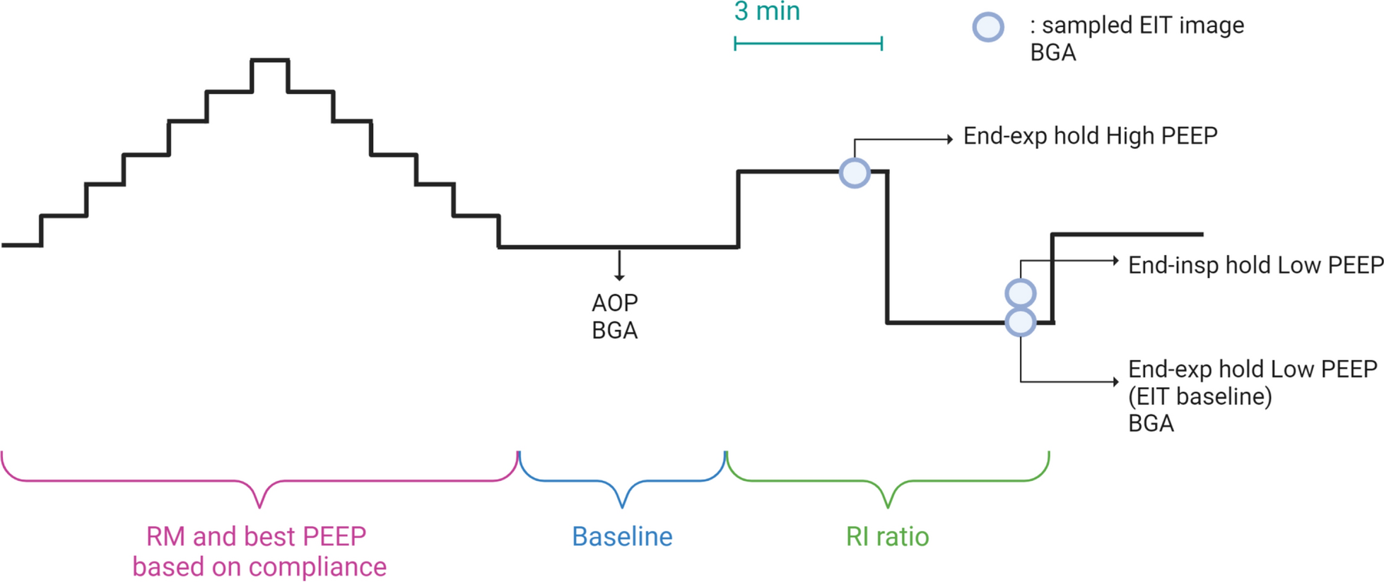
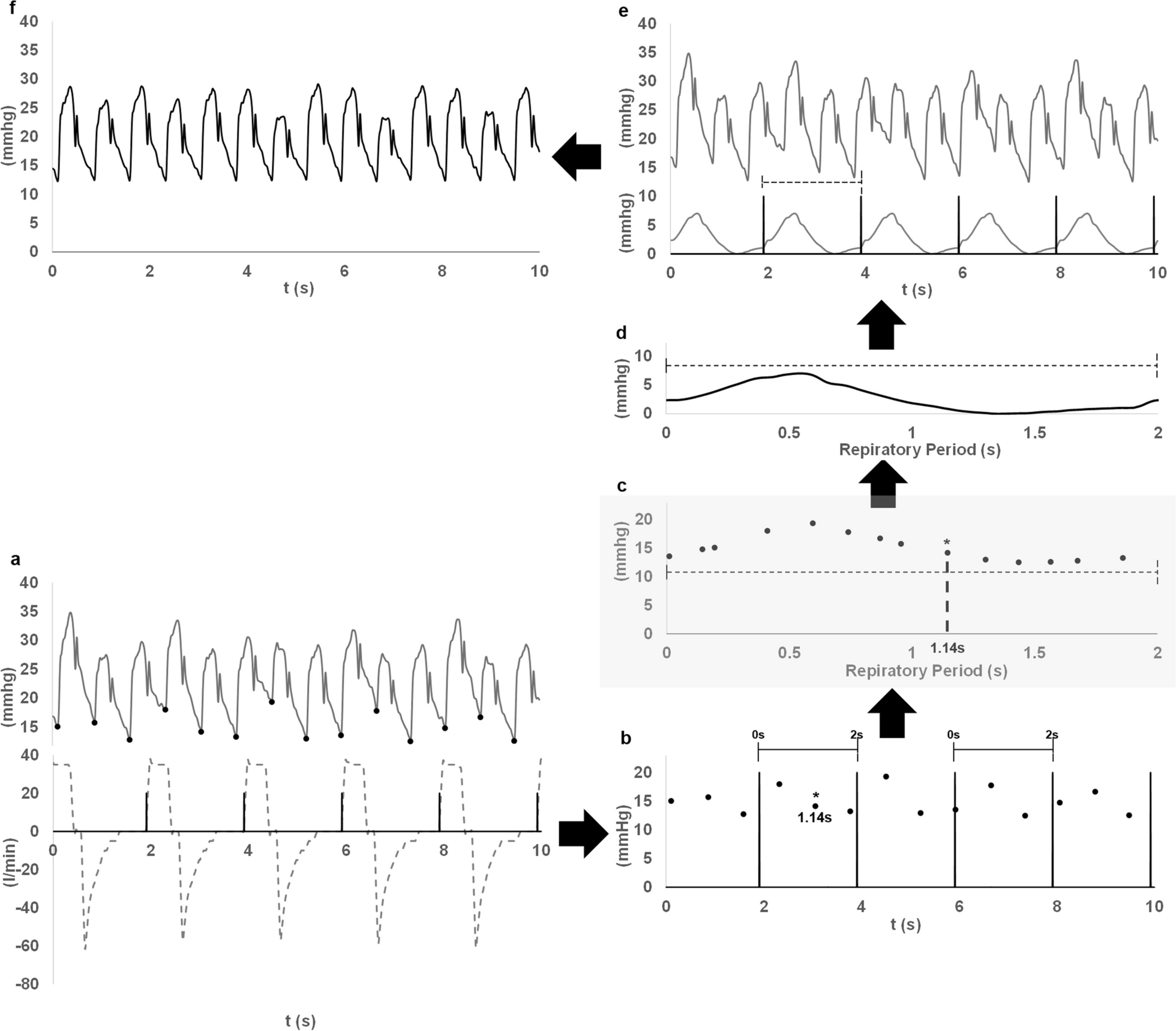
To discern the direct impact of MV on PA waveform, we performed the following steps (Fig. 1):

1)

We identified the minimum pressure at the foot of each PA pressure cycle using an iterative algorithm and the electrocardiogram as fiduciary signal to separate the cardiac cycles (Fig. 1a).

2)

Simultaneously, each respiratory cycle was identified using the airway flow signal and setting a threshold of 5lpm for defining the beginning of the inspiration (Fig. 1a).

3)

The time scale was then adjusted to start at each respiratory cycle initiation (Fig. 1b).

4)

The beginning of each cardiac cycle was marked according to the new time scale, i.e. according to the relative position of the minimum pressure in the respiratory period (Fig. 1b).

5)

Subsequently, cardiac beats were rearranged based on the timing of the minimum pressure value in relation to the respiratory cycle (Fig. 1c). This procedure implies using the respiratory period in the x axis instead of the time scale.

6)

Using these reordered values, we constructed a function that represents the minimum pressure points across the respiratory period. An interpolation technique using a smoothing splines algorithm was applied to estimate missing values ensuring a degree of signal smoothness without significantly altering the primary curve shape (Fig. 1d).

7)

Signal was then scaled by subtracting its lowest value and applying this adjusted function throughout the evaluation timeframe at intervals demarcated by the respiratory cycle (Fig. 1d, e).

8)

In the final step, we subtracted this signal from the recorded PA pressure waveform (Fig. 1e), yielding the corrected PA pressure signal (Fig. 1f). An example of the non-corrected and corrected PA pressure signals in relation to the airway pressure is shown in Additional file 1: eFigure1.

Fig. 1

Algorithm to correct the effect of breathing on pulmonary artery pressure signal. See the description in the manuscript. As noted, the respiratory and pulmonary artery pressure signals should be recorded simultaneously. In brief, the following steps are shown: a minimum pressure (black points) at the start of the pulmonary artery pressure (continuous grey line) cycle and the start of inhalation (black lines) in the respiratory flow (dashed grey lines) cycle are located. b Time of minimum pulmonary artery pressure points in relation with the respiratory cycle period are set (dashed lines demark the respiratory period). One of the minimum pulmonary artery pressure points is marked with a star and its relative position according to the respiratory period is shown. c Minimum pulmonary artery pressure points are reordered according to their relative position in the respiratory cycle. This step is highlighted in grey due to its relevance for the method. The new location of the point marked with a star in b is now shown as an example of this step. d Function of the minimum pressure vs it relative time in the respiratory period is created. The function is scaled to its minimum value. Dashed line demark the respiratory period. e Function is used to create the continuous signal (bottom continuous grey line) along the analysed period and subtracted from the original pulmonary artery pressure signal (top continuous grey line). The dashed line demarks the respiratory period. f Corrected pulmonary artery pressure results from the above mentioned subtraction

Signal acquisition and processing is further described in the online supplement.

Beat-to-beat measurement of RVSV and PAPWA variables for its estimation

On a beat-to-beat basis, the following variables were calculated on PA flow or pressure signals:

Stroke volume reference (SVref): Area under the flow-time curve during systole.

PA pulse pressure: The difference between PA systolic and foot pressure.

PA pressure systolic area: Area under the PA pressure curve, starting at pressure foot and concluding at the dicrotic notch.

PA pressure standard deviation: Pressure SD throughout each pressure cycle.

A detailed description of the methods applied to calculate these variables is provided in the online supplement (Additional file 1: eFigures 2 and 3). Although such methods have been originally developed for systemic arterial pulse wave analysis, the physiological principle, where they grounded should theoretically stand for the PAPWA as well. We assessed the performance of SV obtained from PA pulse pressure (SVPP), systolic area (PASystAUC) and standard deviation (SVSD) derived from both the non-corrected and corrected pressure signals in tracking RVSV.

Evaluation of the impact of breathing on beat-to-beat tracking of RVSV using PAPWA

When using pulse pressure, standard deviation and systolic pressure area for SV estimation by pulse wave analysis, a calibration factor is required [1]. This factor depends mainly on vascular properties, and it is assumed to be constant along the respiratory cycle [9]. In our study, this calibration factor was derived from the ensemble average of 10 PA pressure and flow consecutive cycles obtained during an expiratory pause at each studied situation. The SV obtained from the resulting mean cycle of flow was divided by the evaluated variable (pulse pressure, standard deviation, and systolic area) calculated from the mean cycle of pressure. The calibration factor was utilized for SV derivation from PAPWA variables on a beat-to-beat basis and was applied for both non-corrected and corrected signals.

The SV variation during a respiratory cycle (SVV) [10] was used to quantify the known effect of heart–lung interactions on SV:

SVV = (SVmax − SVmin)/[SVmax + SVmin)/2] [11]where SVmax and SVmin are the maximum and minimum SV during a respiratory cycle. The SVV was calculated for PAPWA SV and for the SVref, computing it for each respiratory cycle over the studied period. The median SVV over the studied period was used as representative of each animal and condition.

For assessing the impact of our correction on the respiratory and cardiac components of the PA pressure signal, a frequency domain analysis was applied. This entailed the generation of an amplitude spectrum on PA pressures segments of 2 min, applying a fast Fourier transform algorithm with a 16,384 size, a Hamming window and 75% overlapping. Noise was defined as a value < 1% of the maximum amplitude of the corresponding spectrum. Respiratory and cardiac components were identified according to the respiratory and heart rates during each study period. The sum of the area under the curve of the 1st–4th harmonics of the respiratory rate was used to calculate the respiratory component, and of the 1st–12th harmonics of the heart rate for the cardiac component.

Statistical analysis

Normalcy was assessed using the Shapiro–Wilk test. Data were expressed as mean (SD) if it followed a normal distribution or otherwise as median [25th–75th interquartile range]. As beat-to-beat SVref and PAPWA variables did not follow a normal distribution during periods of analysis, median was chosen as representative of each animal and condition. Similarly, the median absolute deviation (MAD) [12] and the MAD divided by median (MAD/MED) were calculated as measures of variability for each animal and condition. Paired t test and Wilcoxon signed-rank test (for non-normally distributed data) were used for comparing measurements in baseline versus ARDS and for comparing non-corrected versus corrected PAPWA variables. Two-way repeated measures ANOVA was applied to evaluate the effect of ventilation correction and lung condition (Baseline and ARDS), on PAPWA derived variables. Pearson’s R (for normal distributed data) or Spearman’s Rho (for non-normal distributed data) were calculated to evaluate the correlation between SVref and PAPWA SV and the SVV calculated from them. Cross-correlation between SVref and PAPWA SV was used to test if the effect of MV on measured PA pressure caused a phase shift between flow and pressure signal. A phase shift was defined as an increase in correlation in any lag between ± 1 and ± 4. McNemar’s test was used to test if the proportion of animals in which a phase shift was observed was different with or without the applied correction. To compare lung condition and the effect of correction, a representative value was obtained for each evaluated variable from each animal and condition during the analysis period (for example, Rho between SVref and SVPP). Then, mean (SD) or median according [25th–75th interquartile range] from the 5 animals at each lung condition was used to perform the corresponding comparisons. It was assumed that the effect of correction was specific for each animal, so the correction function was calculated for each individual and situation. However, to characterize the impact of the proposed correction method on the evaluated data set, a mixed effect linear regression of all the measures was used using SV obtained from PAPWA as the dependent variable, SVref, correction and lung condition as fixed effects, and animal as random effect. A Bland–Altman analysis corrected for repeated measurements [13] of all the comparison pairs was performed at each lung condition and the percentage error [14] was calculated to represent the change in agreement caused by the introduction of the correcting method. Significance was considered at p < 0.05. Bonferroni correction was applied to account for multiple comparisons. Statistical analysis was performed with Microsoft excel 2013 (Microsoft Corporation, Redmond, WA, USA) and Stata v15 (StataCorp, College Station, TX, USA).