Database

The NHANES consists of a series of surveys by the National Center for Health Statistics, a division of the Centers for Disease Control and Prevention (CDC), to evaluate the health and nutritional status of civilian, noninstitutionalized U.S. children and adults and to determine the burden of major diseases and their risk factors [26, 27]. In the NHANES, stratified multistage cluster sampling is used with oversampling [28] of specific groups. Demographic, socioeconomic, and nutritional data are collected through in-person interviews, physical examinations and laboratory tests [29]. Recent waves of NHANES data have over-sampled low-income persons, adolescents 12–19 years, individuals ≥ 60 years of age, African Americans, and Mexican Americans. Beginning in 2007–2008, NHANES oversampled all Hispanics, instead of only Mexican American, low-income persons, individuals ≥ 60 years of age, and African American individuals [28]. In addition, the “Asian” group was oversampled after 2011. The original study was approved by an Institutional Review Board with informed consent provided by all study participants.

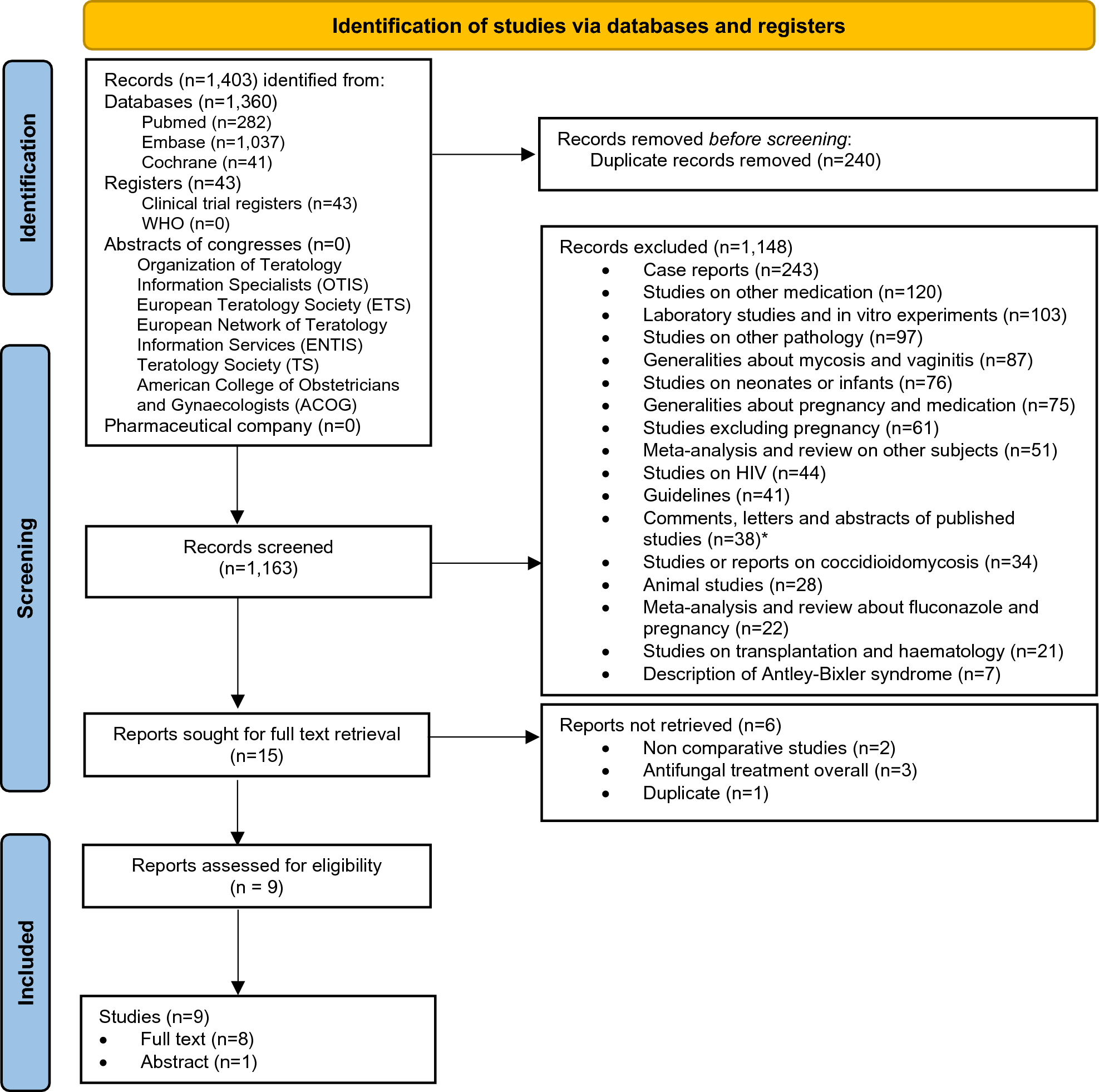
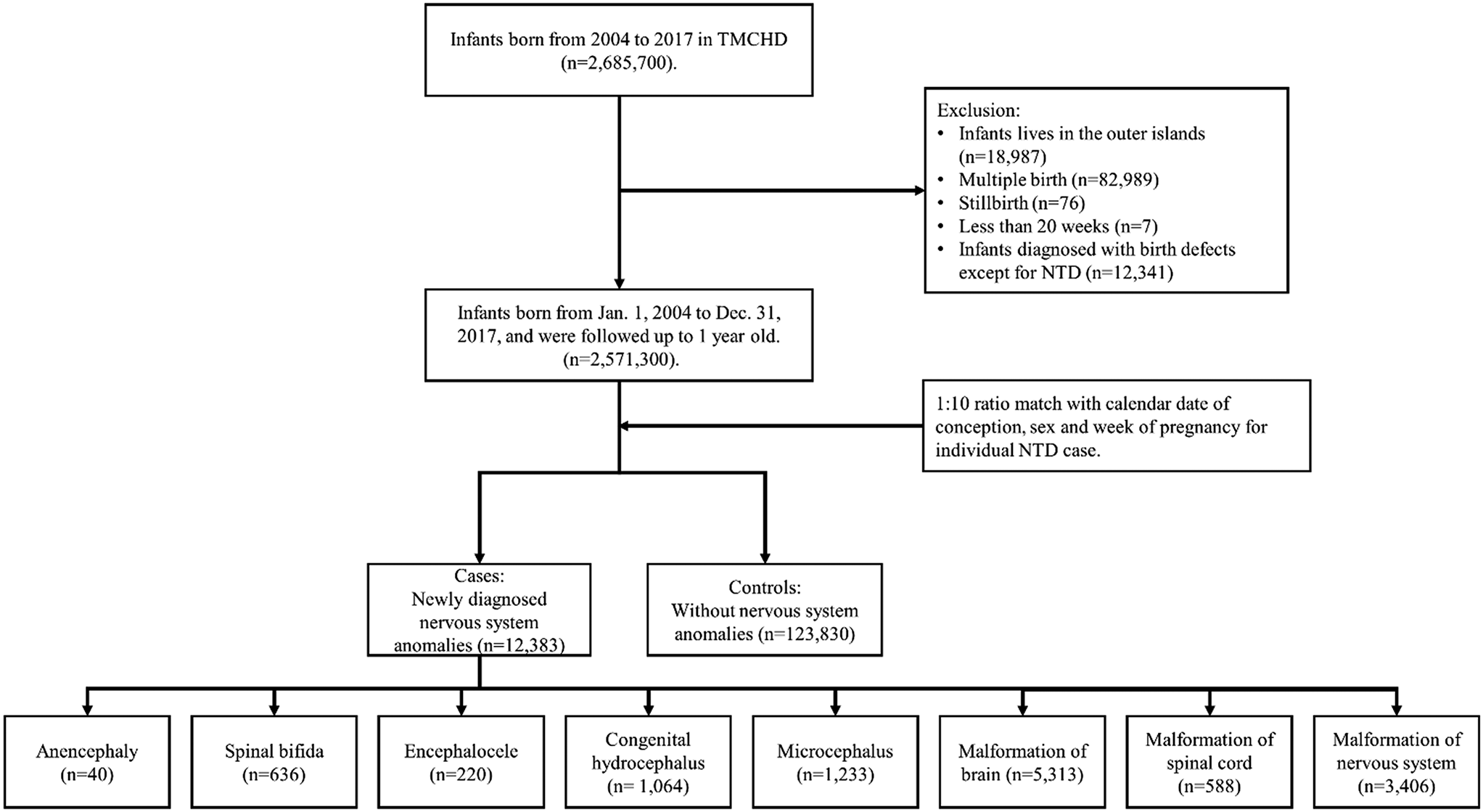
Study sample

The NHANES has been a continuous surveillance system, since 1999. For this study, the initial sample consisted of 10,175 NHANES participants from a single wave (2013–2014). Participants who were < 20 years of age (n = 4,406) were excluded, retaining 5,769 with age range of 20-85y at baseline examination. Of this subgroup, 3,698 were excluded for having missing data on serum NfL. Thus, the final sample consisted of 2,071 adults, ≥ 20 years of age, with complete data on serum NfL. No other exclusions were made for most analyses and all other covariates included in our analyses were imputed, using chained equations [30, 31] with details provided under “Statistical analysis” section (Fig. 1). On average, covariates aside from NfL were missing on 3–4% of the final sample of N = 2,071.

Fig. 1

Participant flowchart: NHANES 2011–2014. Abbreviations: NfL = Neurofilament Light Chain; NHANES = National Health and Nutrition Surveys

Mortality linkage

The National Center for Health Statistics (NCHS) has linked data collected from several NCHS population surveys with death certificate records from the National Death Index (NDI). In compliance with requirements to protect the confidentiality of the NCHS survey participants, restricted-use versions of the linked mortality files are made available only through the NCHS Research Data Center (RDC). To complement the restricted-use files and increase data access, NCHS also developed public-use versions of the linked mortality files for the 1999–2014 National Health and Nutrition Examination Survey (NHANES) among others. The public-use linked mortality files include a limited set of variables for adult participants only. To reduce the participant disclosure risk, the public-use versions of the NCHS linked mortality files were subjected to data perturbation techniques. Synthetic data were substituted for follow-up time and underlying cause of death for select records. Information regarding vital status was not perturbed. The public-use linked mortality file provides mortality follow-up data from the date of survey participation through December 31, 2019. Detailed description of the linkage methodology and analytic guidelines can be found on the NCHS Data.

Linkage webpage: https://www.cdc.gov/nchs/data/datalinkage/LMF2015_Methodology_Analytic_Considerations.pdf

Serum neurofilament light chain measurement

Eligible NHANES 2013–2014 participants who were aged 20–75 years consented to store their blood samples for future research and consisted of individuals who had stored surplus or pristine serum samples. Using a highly sensitive methods, NfL was measured by immunoassay using acridinium ester (AE) chemiluminescence and paramagnetic particles. This assay can be conducted on an existing, high-throughput, automated platform (Attelica). Strict quality assurance was applied and subsample weights were generated to analyze the data properly. The lower and upper limits of quantification were 3.9 pg/mL and 500 pg/mL, respectively. Other details are provided elsewhere (https://wwwn.cdc.gov/Nchs/Nhanes/2013-2014/SSSNFL_H.htm).

Covariates

Socio-demographic characteristics were defined as follows: age (in y), sex (M/F), race (Non-Hispanic White, Non-Hispanic Black, Mexican American or other Hispanic, and Other race/ethnicities including Non-Hispanic Asian), level of education (< 9th grade or High school, 9–11th Grade, HS graduate, GED or equivalent, some college or Associate’s degree, ≥ College Graduate), marital status (married and/or living with partner vs. other) and poverty status as indicated by the poverty-income ratio [PIR] (< 100%, ≥ 100% to < 200% and ≥ 200%). Lifestyle characteristics were focused on smoking status (non-smoker vs. ex-smoker vs. current smoker), alcohol consumption ≥ 12 glasses (in past 12 months) [Y/N], ever use marijuana, cocaine, heroin or methamphetamine (Y/N). Physical activity in the past 30 days (moderate activity or vigorous activity, work or leisure; walk or bicycle) using a set of self-reported responses based on the short form of the International Physical Activity Questions [32] in terms of frequency (# of days) per week and number of minutes per day. Those were then combined to generate MET.min/week for each category of physical activity intensity. Finally, the MET.min/week values were added together. The NHANES 2013–14 included a dietary component consisting of two 24-h recalls administered by trained Mobile Examination Center (MEC) interviewers. The U.S. Department of Agriculture (USDA) by computerized Automated Multiple Pass Method was used to collect dietary intake data [33]. The first dietary recall interview was collected in-person in the MEC and the second interview was collected by telephone 3 to 10 days later. Nutrient intakes were estimated by linking dietary intake with corresponding USDA’s Food and Nutrient Database for Dietary Studies databases [34, 35]. The average daily nutrients intake from the two 24-h recalls was used in our current analysis. In our present study, the formula reported by Mellen et al. [36] was used to calculate the DASH diet score. This score is divided into nine target nutrients, specifically total fat, saturated fat, protein, fiber, cholesterol, calcium, magnesium, sodium and potassium. Micronutrient goals were expressed per 1000 kcal. The total DASH score was based on the sum of all nutrient targets met. If the participant achieved the DASH target for a nutrient, a value 1 was assigned. A value of 0.5 was given if the intermediate target was achieved, while a value of zero was assigned if neither target was met. Each of the nine components of the DASH total score were considered as separate exposures in our current study, in addition to the total score. In addition to dietary intakes, 3 nutritional biomarkers were included among potential confounding covariates, namely RBC folate, serum vitamin D3 [25(OH)D3] and serum vitamin B-12. Those are described in more detail in supplementary methods 1. Health characteristics were considered among potential mediators/moderators in the association between serum NfL and all-cause mortality. Those included body mass index (BMI) categories, self-rated health (SRH), a co-morbidity index and several measures of cardiometabolic health: systolic and diastolic blood pressure (mm Hg., average of 3 readings), glycated hemoglobin (HbA1c), total cholesterol and urinary albumin:creatinine ratio, ACR (Loge transformed with outliers excluded), (supplementary methods 1). The co-morbidity index was a binary [Y/N] variable for any of several cardio-vascular and cancer morbidities, namely congestive heart failure, coronary heart disease, angina/angina pectoris, heart attack, stroke or cancer/malignancy. SRH was operationalized by one question: “Would you say your health in general is- excellent, very good, good, fair or poor?” and further dichotomized as “excellent/very good/good” as the referent category (“0”) vs. “fair/poor” coded as “1”.

Statistical methods

We used Stata release 17 [37] to perform all descriptive and inferential analyses, accounting for sampling design complexity by including sampling weights, primary sampling units and strata in parts of the analyses. Aside from outcome and exposures, data was imputed using chained equations or MICE (5 imputations, 10 iterations) [30, 31], with most covariates having < 10% missing data compared to the final eligible sample (i.e. N = 2,071). MICE is a statistical technique that iteratively generates multiple imputations for each missing value in a dataset [30, 31]. This is accomplished by fitting predictive models to the observed data and assigning missing values progressively, one variable at a time, using information from other variables [30, 31]. A predictive model is created for each incomplete variable, using observed values of other variables to approximate the missing values [30, 31]. The imputation procedure is continued for a set number of iterations, typically until convergence is reached [30, 31]. At each iteration, missing values are updated using the most recent imputations, allowing imputation models to be refined [30, 31]. In our study, this is done for 10 iterations per imputation for a total of 5 imputations. Main Stata commands used included mi impute, mi passive and mi estimate in all the analyses. Study design complexity and survival time setting was specified using mi stset and mi svyset among others. Only potentially confounding and mediating/moderating covariates were imputed within the final selected sample with complete exposure and outcome data. The overall analytic sample was characterized at baseline using means and proportions. A series of bivariate and multivariable regression models were constructed to evaluate whether baseline characteristics varied according to sex, while accounting for sampling design complexity. To examine associations among plasma NfL exposures, we estimated a series of Cox proportional hazard regression models with sequential covariate adjustment. Time on study (months) was used as the initial underlying scale and was used to generate age at death accounting for initial age at baseline assessment in the NHANES. Sex-specific Kaplan–Meier survival curves were presented for binary NfL exposures (> vs. ≤ median) based on distributions in the final selected sample that has a cutoff of 2.51 for NfL on the Loge transformed scale, while examining time on study as the analytic time variable. In Cox proportional hazards models, heterogeneity by sex of the association between NfL exposures and mortality was tested through addition of two-way interaction terms (NfL × sex) in separate models. The same models were also stratified by sex. Similarly, and as a secondary analysis, interaction by baseline age was tested for the main exposure, overall and within each gender group. The general modeling strategy consisted of a basic model, adjusted for age, sex, race and PIR (Model 1), to which other lifestyle and health-related covariates (listed in the Covariates section) were subsequently added (Model 2).

BMI, measures of cardio-metabolic health (SBP, DBP, total cholesterol, HbA1c and ACR), co-morbidity index, self-rated health and nutritional biomarkers (RBC folate, serum 25(OH)D3, and serum vitamin B-12) were separately assessed as mediating/interactive factors in the total effect of NfL exposures on all-cause mortality in the full Model 2. All other covariates in Model 2 as previously described were considered potential confounders. Continuous potential mediators were transformed into standardized z-scores, while indices were coded as 0 = no, 1 = yes/any, for ease of interpretation. Specifically, the overall effect of each main exposure on all-cause mortality (Y), in the presence of a mediator with which the exposure a may interact (M), was decomposed into four distinctive components, using the following general form of the model, accounting for potentially confounding covariates c [38]. Therefore, in all analyses, exposure levels were a = 1 and a’ = 0.

$$\begin E\left[ \right)} \right] = \theta_ + \theta_ a + \theta_ m + \theta_ a*m + \theta_ c \hfill \\ E\left[ \right)} \right] = \beta_ + \beta_ a + \beta_^ c \hfill \\ \end$$

(i)

Neither mediation nor interaction or controlled direct effect (CDE): E[CDE | c] = θ1 (a–a’). This component is interpreted as the effect of the exposure on the outcome, not related to interaction or mediation [38].

(ii)

Interaction alone (and not mediation) or interaction reference (INTref): E[INTref | c] = θ3(β0 + β1a’ + βcTc)(a–a’). This component is interpreted as the interaction effect of the exposure on the outcome in the presence of the mediator, when the presence of the outcome is not necessary for the presence of the mediator [38].

(iii)

Both mediation and interaction or mediated interaction (INTmed): E[INTmed | c] = θ3 β1 (a–a’)(a–a’). This component is interpreted as the interaction effect of the exposure on the outcome in the presence of the mediator, when the presence of the outcome is necessary for the presence of the mediator [38].

(iv)

Only mediation (but not interaction), or pure indirect effect (PIE): E(PIE | c] = (θ2 β1 + θ3 β1a’)(a-a’). This component is interpreted as the effect of the mediator on the outcome when the exposure is necessary for the presence of the mediator [38].

The total effect of the exposure on the outcome (TE = CDE + INTref + INTmed + PIE), is the summation of those four partitioned components that explain the total variance between the exposure and the outcome [38]. This four-way decomposition unifies methods that attribute effects to interactions and methods that examine mediation, and this method has recently been introduced in Stata, allowing to estimate four-way decomposition using parametric or semi-parametric regression models. Importantly, the Med4way command [39] [https://github.com/anddis/med4way] was used to test mediation and interaction of the total effects of NfL exposure on mortality with several mediators/effect modifiers, using Cox PH models for the outcome and linear or logistic regression models for each mediator/effect modifier. In this study, four-way decomposition was applied to the total sample. A logit link was specified for the mediating variable equation when mediators were binary. Total effects were interpreted as hazard ratios on the Loge scale based on Cox proportional hazards models, per SD of exposures if the exposure was continuous and for “exposed” vs. “unexposed” if the exposure was binary. These total effects were then decomposed into four components. An effect size that would result in a hazard ratio > 1.5 was considered as moderate-to-strong. Unlike all other analyses, four-way decomposition models did not account for sampling design complexity.

In all models, we adjusted for sample selectivity due to missing exposure and outcome data, relative to the initially recruited sample, using a two-stage Heckman selection strategy [40]. Initially, we predicted an indicator of selection with socio-demographic factors, namely, age, race, sex and PIR using probit regression, which yielded an inverse mills ratio (IMR)—a function of the probability of being selected given those socio-demographic factors. Subsequently, we estimated our Cox proportional hazards regression models adjusted for the IMR in addition to afore-mentioned covariates [40, 41].

Two supplementary analyses were also carried out. In a first supplementary analysis, all variables of interest including potential mediators/moderators and exogenous variables were compared across exposure levels (above vs. below median) using bivariate linear and multinomial logistic models on multiple imputed data. The second supplementary analysis specifically examined the association between each potential moderator with all-cause mortality (multivariable-adjusted Cox PH model with only main effect of the potential moderator: Model A); tested interactions between Loge transformed and z-scored NfL and those variables of interest in relation to all-cause mortality (multivariable-adjusted Cox PH model with 2-way interaction between NfL and each potential moderator: Model B); and associations of potential mediators/moderators with NfL while adjusting for exogenous covariates (multiple linear regression models, multiple-imputed data: Model C). In Model B, interaction was tested on the multiplicative scale. Conversion to the additive scale can be implied with equations shown below for the Cox proportional hazards model and the relative excess risk due to interaction (RERI), when both exposures and moderators are binary [42,43,44]. This sub-analysis was carried out with exposure (LnNfL, z-scored) and continuous moderators transformed into below and above median binary variables, as well as the remaining binary potential moderators. RERIHR formula is shown below with IR being the estimated incidence rates within each group, conditioning simultaneously on exposure and potential moderator [42,43,44]. For each combination of exposure and potential moderator level, an excess relative risk was computed as shown below [42,43,44]. The attributable proportion (AP) statistic is the proportion of risk for the doubly exposed (+ + or 11) interaction that is due to the risk that is above additive. The synergy index (SI) statistic is the excess risk expressed as a ratio rather than a difference, with a value > 1 indicating synergy or super-additive effects [42,43,44]. Exogenous covariates included age, sex, race/ethnicity, PIR, education, smoking, ever drug use, alcohol use, DASH, total caloric intake, physical activity, household size and marital status. All Stata codes used and secondary Output in this study will be provided under the following repository: baydounm/NHANES_NfL_mortality (github.com).

$$\lambda (t;X,M,C) = \lambda_ (t)e^ X + \beta_ M + \beta_ XM + \sum\limits_^ C_ } }}$$

$$\begin RERI_ = e^ + \beta_ + \beta_ }} - e^ }} - e^ }} + 1 = HR(1,1;c) - HR(1,0;c) - HR(0,1;c) + 1 \hfill \\ = \frac - IR_ - IR_ + IR_ }} }} \hfill \\ \end$$

$$ERR = IR_ /IR_ - }\;a\;}\;m\;} 0 \, \left( - \right)}\left( + \right).$$

$$\begin AP = RERI_ /IR_ \hfill \\ SI = \left( - 1} \right)/\left[ - 1} \right) + \left( - 1} \right)} \right] \hfill \\ \end$$