Postmortem human tissue samples

In total, we examined 15 snap-frozen tissue blocks, obtained from autopsies from six people diagnosed with MS and seven tissue donors without recognizable neuropathological changes (CTRL). All tissue samples used in this work were provided by the UK Multiple Sclerosis Tissue Bank at Imperial College London, after ethical approval by the National Research Ethics Committee in the UK (08/MRE09/31). Further information about the donors is provided in Supplementary Table 1. No statistical methods were used to predetermine sample size but our sample size is similar to those reported in previous publications, for example Absinta et al.5 and Schirmer et al.23. Data collection and analysis were not performed blind to the conditions of the experiments.

IHC and histochemistry

Snap-frozen tissue blocks were dissected into 16-µm-thick sections using a Leica Microsystems CM3050S cryostat, placed on VWR superfrost plus microscope slides and stored at −80 °C. Histopathological assessment was performed using IHC for CD68 and CD163 as described previously23. The following antibodies were used: mouse anti-CD68 (cat. no. 333802, 1:200, Biolegend), and mouse anti-CD163 (cat. no. NCL-L-CD163, 1:1,000, Novocastra).

For chromogenic CD163 IHC and histochemistry, tissue sections were fixed on slides by thawing and drying, followed by immersion in acetone for 10 min at 4 °C. Afterwards, slides were allowed to dry at room temperature. CD163 was stained with an Autostainer Link 48 by Dako. Endogenous peroxidase was blocked using a ready-to-use peroxidase-blocking solution (cat. no. S202386-2, Dako). The primary antibody was diluted in antibody diluent (cat. no. S080983-2, Dako) and applied for 60 min at room temperature. After a washing step, slides were exposed to a mouse-specific biotinylated secondary antibody (cat. no. GV82111-2, Dako) for 15 min, followed by incubation with streptavidin-linked horseradish peroxidase (cat. no. SM802, Dako) for 20 min. The staining was developed using a 1:50 dilution of 3,3′-diaminobenzidine (DAB) chromogen in DAB+ substrate buffer (cat. no. GV825, Dako) for 10 min. Sections were counterstained using hematoxylin and eosin (H&E) and coverslipped.

Sections were stained for myelin with LFB by incubation with 0.1% LFB at 56 °C overnight. After washing with 96% ethanol and rehydration, the slides were immersed in 0.1% aqueous lithium-carbonate solution for 5 min. The staining was differentiated in 70% ethanol until the myelin sheaths obtained an intense blue color. Subsequently, tissue slides were washed with distilled water, counterstained with periodic acid-Schiff and, following dehydration, coverslipped with a mounting medium (cat. no. 03989, Merck).

To localize ferrous and ferric iron, DAB-enhanced Turnbull Blue (TBB) was applied as described previously66. In short, the slides were dried and exposed to 10% ammonium sulfide solution (cat. no. 105442, Merck) in double-distilled water for 90 min. Consecutively, slides were immersed in 10% potassium ferricyanide and 0.5% hydrogen chloride in an aqueous solution for 15 min. This step was followed by blocking the endogenous peroxidase with 0.01 M sodium azide and 0.3% hydrogen peroxide in methanol for 60 min. The slides were washed with 0.1 M Sorensen’s phosphate buffer and the staining was developed with a 1:50 solution of DAB chromogen (cat. no. K3468, Dako) and 0.005% hydrogen peroxide in Sorensen’s phosphate buffer for 20 min. Slides were counterstained with H&E and coverslipped.

For IF staining, sections were fixed in ice-cold methanol, 4% paraformaldehyde or acetone at room temperature for 10 min, then blocked with PBS-T (PBS 1×, Triton 0,1%) and goat serum (cat. no. 16210-064, Gibco, 1:10) for 30 min. Primary antibodies were diluted in PBS-T or Intercept-TBS (cat. no. 927-60001, LI-COR) and then incubated overnight at 4 °C. The slides were washed twice with PBS for 5 min and then incubated with secondary antibodies diluted in PBS-T for 2 h. Slides were then washed twice with PBS for 5 min and mounted using Fluoromount-G with 4,6-diamidino-2-phenylindole (DAPI) (cat. no. 00-4959-52, ThermoFisher Scientific). The following primary antibodies were used: rabbit anti-SPAG17 (cat. no. PA5- 55912, ThermoFisher, 1:100), mouse anti-SMI32 (cat. no. 801701, Biolegend, 1:2,500), rat anti-GFAP (clone 2.2B10, cat. no. 13-0300, ThermoFisher, 1:200), rabbit anti-CD3 (clone CD3-12, cat. no. MCA1477, Bio-Rad, 1:200), rabbit anti-CD11B (clone EPR1344, cat. no. ab133335, Abcam, 1:500) and mouse anti-CD19 (clone HIB19, cat. no. 302202, Biolegend, 1:50). Separate slides were stained only with secondary antibody, to be able to identify background signals.

Fluorescence multiplex in situ RNA hybridization

For smFISH validation, we processed cryosections of 14 µm thickness. smFISH was performed on a representative selection of CTRL and MS tissue samples using ACD RNAscope 2.5 HD Red and Multiplex Fluorescent v.2 assays (ACD Biotecne), following the protocol of a previous publication1. The following human RNAscope assay probes were used: HMGB1 (C1), SPAG17 (C1), CD14 (C1), CD163 (C2), TLR2 (C2), ITGB1 (C2), ADCY2 (C3) and VWF (C3). For multiplex ISH, probes were labeled with TSA Vivid Fluorophores (Fluorescein, Cyanine 3, Cyanine 5, Akoya Biosciences). Slides with positive ISH and human ACD bio-techne 3-plex negative probes, were used in every run as quality control.

Image acquisition and quantification

Brightfield images of CD163, CD68, TBB (iron) and LFB were acquired using a Leica DM6 B microscope with Leica K3C camera at ×20 magnification. Pictures were imaged with the Leica Application Suite X (LAS X) software (v.3.8.1.26810) and exported as TIFF files and later processed using ImageJ (v.2-2.14.0) software. Images were also acquired using Hamamatsu NanoZoomer 2.0HT at ×40 magnification and exported as NPD files. Image processing of histological data was performed using GIMP-v.2.10 software.

Multiplexed fluorescent images were taken using a Leica DM6 B microscope with a Leica K5 camera, and preprocessed with a thunder imaging system. Focus points were set at ×20 magnification for overview and quantification purposes. All fluorescent pictures are z-stack images consisting of 10–20 layers with a 0.7-μm step size, in all four channels. Pictures were imaged with the LAS X software, exported as LIF files and analyzed with QUPATH (v.0.4.3)67. First, cells were detected on the DAPI channel. Cell expansion was set at 2 µm, and subcellular spot detection was run for ADCY2 and SPAG17. Double positive cells were classified using a composite classifier on the estimated subcellular spots of ADCY2 and SPAG17. Quantification was performed for LC, LR and PPWM lesion areas.

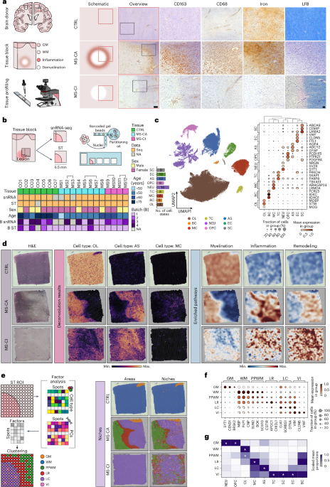
Histopathological assessment and lesion type characterization

We focused on subcortical WM specimens for analysis; however, in certain cases, small adjacent GM areas have been captured during tissue sectioning. WM lesions were identified as areas with a marked loss of myelin staining visualized through LFB-periodic acid-Schiff histochemistry. We further classified lesions by IHC using antibodies against CD68, CD163 to detect activated MC and TBB to detect iron at LRs. Lesions were then classified into MS-CA or MS-CI according to established criteria12. Notably, fully remyelinated lesions, so-called shadow plaques, were not included. Staging of lesion types was performed by a trained neuropathologist specializing in MS pathology. Chronic active lesions showed a hypocellular, demyelinated lesion center but a distinct inflamed rim with presence of CD68- and CD163-positive cells, regularly containing LFB-positive myelin degradation products. Some of these lesions showed accumulation of iron-laden microglia and macrophages at the rim. Chronic inactive lesions were characterized by a fully demyelinated, hypocellular lesion center, a low frequency of CD68- and CD163-positive macrophages or microglia within lesions and a distinct rim without accumulation of CD68- or CD163-positive cells.

Sample selection for transcriptomics

The RNA integration number (RIN) was used as a sample selection criteria, and only samples with a value of ≥5.9 were included for both transcriptomic analysis. We cut 70-µm-thick sections of tissue on a Leica Microsystems CM3050S cryostat to obtain a final weight of 15 mg of tissue, from which the RNA was isolated. This was done using TRIzol (cat. no. 15596026, ThermoFisher), chloroform (cat. no. 1731042, Sigma Aldrich) and RNeasy mini kit (cat. no. 74104, QIAGEN) following the manufacturer’s recommendations. RNA integrity was measured on an Agilent 2100 Bioanalyzer using the High Sensitivity RNA ScreenTape (cat. no. 5067-5579, Agilent), buffer (cat. no. 5067-5580, Agilent) and ladder (cat. no. 5067-5581, Agilent) according to the manufacturer’s instructions.

Nuclei isolation, library preparation and ambient mRNA correction

Nuclei from selected samples were isolated using sucrose-gradient ultracentrifugation according to established workflows23. Following isolation, nuclei were diluted to a final concentration of 1,000 nuclei per microliter and loaded to the 10x Genomics Chromium controller aiming for a recovery rate of 8,000 nuclei per sample. We prepared the libraries following the 10x Genomics protocol using the 3′ single cell v.3.1 kit (cat. no. PN 1000121) with single indexing. Samples were sequenced on a NovaSeq 6000 aiming for a sequencing depth of 30,000 reads per nucleus. Expression count matrices for each sample were generated using Cell Ranger Count (v.6.0.2) by performing alignment to the sequencing data against the GRCh38-2020-A reference transcriptome. Then, the obtained count matrices were corrected for ambient mRNA using CellBender (v.0.2.0)68 with the following parameters: model = full; expected_cells = 8,000; total_droplets_included = 50,000; fpr = 0.01; epochs = 150; posterior_batch_size = 5; cells_posterior_reg_calc = 50.

snRNA-seq data quality control

The data processing and downstream analyses for the snRNA-seq datasets was done using the scanpy toolkit (v.1.9.6)69 in Python (v.3.10.0). Each sample was filtered separately to control for batch differences. Single nuclei were filtered by genes (<200 genes), mitochondrial genes (percentage of mitochondrial genes <5%) and gene counts (number counts < number counts 99th percentile). Genes were kept if they were expressed across different nuclei (number of expressed nuclei >3). Afterwards, nuclei were filtered by doublet scores computed with scrublet70 (doublet score <0.1). Finally, each nuclei raw expression was normalized by the median of total counts (target_sum = None) and log-transformed (log1p).

snRNA-seq data integration and cell annotation

A single AnnData object was generated by concatenating (join=outer) all preprocessed nuclei coming from different samples. Feature selection was performed by computing high variable genes per sample and then selecting the top 4,096 genes that were flagged as variable in the maximum number of samples. Genes were then scaled across nuclei and principal component analysis (PCA) was calculated on the selected features. Harmony-py (v.0.0.9)71 was used to integrate the obtained PCs, eliminating batch effects between samples. Nearest neighbors were generated for nuclei by estimating similarities in the PC space (n_pcs = 50). The connectivities obtained were used to generate a uniform manifold approximation and projection (UMAP) manifold. Nuclei were clustered using the Leiden graph-clustering method72 (resolution = 0.25) and annotated manually using brain gene markers5,23 (Supplementary Table 3).

Comparison with an independent atlas

To validate cell type annotation, we compared our generated atlas with another reference human snRNA-seq atlas at the molecular level5. The count matrix and annotation metadata were downloaded from GSE180759. Pseudobulk transcriptomic profiles were generated for both atlases at the cell type level using decoupler-py (v.1.5.1, commit b6b430e)73. Then, genes were filtered based on the following hyperparameters: min_count = 10, min_total_count = 15, min_prop = 0.2, min_smpls = 2. To make them comparable, we filtered the profiles by the intersection of genes between the two atlases and log-normalized them with scanpy (target_sum = None). Finally, the Pearson correlation between the different profiles was performed and the P value adjusted by Benjamini–Hochberg (BH) correction (BH-adjusted P < 0.05; r > 0.75).

Identification and characterization of cell subtypes

To identify cell subtypes of principal cell lineages, the main cell types were subsetted from the entire snRNA-seq atlas. Genes with enough expression across cell types were kept (number of expressed nuclei >3), and samples with not enough cells for a particular cell type were removed (number of cells ≤5). PCA was then performed on the scaled log-transformed most variable genes across as many samples as possible. Depending on the number of cells, different numbers of variable genes were used: 4,096 genes (number of cells >1 × 104), 2,048 genes (number of cells >1 × 103) and 1,024 genes (number of cells <1 × 103). PCs were integrated using harmony-py71, nearest neighbors were computed per nucleus by finding similarities in the corrected PC space (n_pcs = 50) and the obtained connectivities were used to generate a UMAP manifold and clustering with the Leiden algorithm (resolution = 1.0). Clusters were characterized by identifying marker genes using the rank_genes_groups (method = t-test_overstim_var) function from scanpy with the log-transformed counts (adjusted P < 0.05; abs(log2FC) > 0.5). Finally, clusters were manually annotated based on marker genes (Supplementary Table 4). Clusters with no clear molecular profiles were removed (denoted as NA).

ST workflow

The 10x Genomics Visium Spatial Gene Expression platform was used for the ST experiments. Tissue samples (RIN ≥ 5.9) were cut into 10 µm sections using a Leica CM3050 S cryostat and placed into a Spatial Gene Expression Slides (cat. no. PN-1000185, region of interest (ROI) 6.5 × 6.5 mm) that was precooled inside the cryostat at −22 °C. The slides were stored in a container at −80 °C until further processing. The sections were then fixed and stained using protocol CG000160 Rev B. The sections were then imaged for a general morphological analysis and for future spatial alignment of the data using a ×10 lens equipped to a Leica DMi8 microscope and processed by LAS X.

Next, slides were permeabilized enzymatically for 18 min. This time was assessed using the 10x Visium Tissue Optimization kit (PN-1000191) and following the protocol CG000238 Rev D. The generation of the libraries was performed according to published protocols (10x Genomics): CG000239 Rev D, using the Gene Expression Reagent kit (cat. no. PN-1000186), the Library Construction Kit (cat. no. PN-1000190) and the Dual Index Plate TT Set A (cat. no. PN-1000215). To assess the correct amplification of obtained cDNA, QuantStudio 3 from ThermoFisher was used. For full length of cDNA and indexed libraries analysis, the TapeStation 4200 analyzer (Agilent) was used. The libraries were loaded at 300 pM and sequenced on a NovaSeq 6000 system (Illumina) with a sequencing depth of 250 million reads per sample.

The data were subjected to demultiplexing using SpaceRanger software (10x, v.2.0.0), creating FASTQ files. These files were then used by SpaceRanger count to perform alignment with the human reference genome GRCh38-2020-A, tissue detection, fiducial detection and barcode/unique molecular identifier counting generating a spatial gene count matrix per slide.

ST data annotation and quality control

First, spatial coordinates were annotated manually by a trained neuropathologist based on myelin (MOG, MBP and PLP1), myeloid cell (CD68) and astrocyte (AQP4, and GFAP) marker staining into different area types using the Loupe Browser v.6.3.0 software (10x Genomics). For each slide, spots were filtered by genes (<200 genes) and genes were kept if they were expressed across different spots (number of expressed spots >3) using scanpy. Finally, raw expression of each spot was normalized by the median of total counts (target_sum = none) and log-transformed.

The lesion area was subdivided into distinct zones. The LC or core covers the demyelinated area surrounded by the LR, which is the distinct border between the demyelinated lesion center and the surrounding myelinated WM, called PPWM. Annotations and delineations of lesion areas were carried out according to a previous publication22.

ST cell type deconvolution

The cell2location (v.0.1.3)74 package was used to calculate cell type abundances for each spot. Based on the annotated snRNA-seq atlas, reference expression signatures of main cell types were inferred leveraging regularized negative binomial regressions. Then, each slide was deconvoluted using hierarchical Bayesian models with the following hyperparameters: N_cells_per_location = 5 and detection_alpha = 20. Afterwards, cell type proportions were calculated per spot by dividing the abundance of a given cell type by the total sum of abundances of a given spot. To check how well the deconvolution worked, we compared the estimated cell type proportions from each slide with the actual cell type proportions in its matching snRNA-seq data. We did this by calculating the Pearson correlation at both the sample and cell type levels. Additionally, spatial activity scores were computed using the enrichment method ULM from decoupler with the REACTOME73,75 pathway genesets (bandwidth = 150).

Generation, characterization and validation of niches in ST data

To annotate niches in an unsupervised way across spots, gene expression and cell type compositions were first integrated into a multiview factor model using MOFA+ (v.0.7.0)26 for each slide independently. Specifically, cell type proportions were transformed to centered log ratios76 using the clr function of the composition-stats Python package (v.2.0.0), while gene expression was summarized into 50 principal components by computing PCA on the scaled top 4,096 variable genes. These two matrices were treated as different views in the MOFA+ model to generate 15 latent factors with the following parameters: scale_views = False, center_groups = False, spikeslab_weights = False, ard_weights = False, ard_factors = False. Then, nearest neighbors were generated per spot by estimating similarities in the latent factor space. The obtained connectivities were used to generate a UMAP manifold and to cluster spots using the Leiden algorithm (resolution = 1.0). Clusters were then annotated manually into niches based on cell type presence and pathway activities of the hallmark genesets77 generated with the enrichment method ULM from decoupler73.

To identify marker genes of niches, slides were concatenated into a single AnnData object and the scanpy’s function rank_genes_groups (method = t-test_overstim_var) was used. Additionally, to identify characteristic cell types per niche, cell type proportions were averaged per slide and then tested for differences against the rest (Wilcoxon rank-sum test, adjusted P < 0.05).

To assess the level of overlap between the computationally annotated niches and the ones annotated by a pathologist, the Jaccard index and the ARI were computed for each slide, ignoring categories that were not shared between annotations. Additionally, similarities between intra and interniche spots were computed using the Pearson correlation at the pseudobulked gene expression and mean clr-transformed cell type proportions.

Neighborhood analysis of spatial niches was performed by computing local spatial proportions. For each slide, a binary matrix (spots as rows and niches as features) was generated based on the obtained niche annotations. Niche binary values per spot were weighted spatially by averaging neighboring spots using an L1-norm Gaussian kernel (bandwidth = 150), obtaining spatial proportions. Values were then averaged per niche across slides.

Spatial trajectory analysis across niches

Slides were concatenated and pseudobulk profiles were generated for each niche and slide combination using decoupler73. Genes were kept following hyperparameters: group = None, min_count > 10, min_total_count > 15. The resulting gene profiles were log-transformed and normalized (target_sum = 1 × 104). The Spearman correlation was then computed for each gene based on the following niche order: WM, PPWM, LR, LC, VI. The obtained gene correlation statistics were then used to infer pathway activities that change differentially across the trajectory from the PROGENy78 resource using the ULM method. Significant pathways (P < 0.05) were then also computed for the pseudobulked gene expression profiles. Finally, the correlated genes, separately for positive and negative, were tested for enrichment for genesets from the REACTOME75 collection using the method ORA from decoupler73. Genesets containing the words FETAL, INFECTION or SARS were removed before computing the enrichment.

Characterization of ciliated AS

Samples and slides containing Ependym, MS11 and MS12 were removed from the analysis due to the similarity of EP cells to ciliated AS. A ciliated AS geneset was obtained by filtering the obtained marker genes with scanpy from the filtered atlas (method = t-test_overestim_var, adjusted P < 1 × 10−4, log2FC > 1). Spots containing AS (proportion > 0.25) were predicted to contain ciliated AS by computing enrichment scores using the obtained geneset with the ULM method from decoupler (weight = None, P < 0.05, score > 0)73. Due to differences in number of spots per slide, a bootstrap strategy was employed to test in which niches ciliated AS are found. For each niche, the total number of spots predicted to contain ciliated AS was used as the estimate. Then, 1,000 random permutations were performed, recording whenever the sampled ciliated AS were higher than the original estimate, to obtain an empirical P value per niche (adjusted P < 0.05). For enrichment analysis, the ciliated AS geneset was tested for enrichment against the REACTOME collection using the ORA method from decoupler (adjusted P < 0.05)73. Genesets containing the words FETAL, INFECTION or SARS were removed before computing the enrichment. Transcription factor activity was computed at both the nuclei and spot level using the CollecTRI79 resource with the method ULM from decoupler73.

Multidimensional scaling of samples

Multidimensional scaling (MDS) implemented in the sklearn (v.1.4.0) Python package was used to capture and visualize sample differences at different levels: cell type proportions, cell subtype proportions, deconvoluted cell type proportions, cell type gene expression and tissue niche gene expression. Cell type, cell subtype and deconvoluted cell type proportions were log-ratio transformed using the clr function of the composition-stats Python package. For gene expression, latent factors capturing shared gene programs between cell types or niches were inferred using the package MOFAcellulaR80 for snRNA-seq and ST samples, respectively.

For snRNA-seq data, we inferred four multicellular factors using multicellular factor analysis80 with MOFA+26 on the pseudobulk expression profiles of each cell type and sample. Each pseudobulk profile was built by summing the gene counts of all cells belonging to a cell type and a sample. Pseudobulk profiles built from at least ten cells were kept in the analysis. Within each cell type, genes expressed in at least 25% of the samples were kept for the analysis. A gene was considered to be expressed in a sample if at least 100 counts were identified. Samples within a cell type with a gene coverage of <90% were excluded. Cell types with fewer than ten samples or greater than 50 genes were not included in the analysis.

For ST data, we inferred three factors using multicellular factor analysis on the pseudobulk expression profiles of each niche and disease sample. Pseudobulk profiles were filtered as described above, except that niches with fewer than nine samples were excluded.

Distances were then computed between samples for each different level by computing the following term: distance = 1 − corr(x, y), where corr is the Pearson correlation coefficient between the vector values of sample x with the vector values of sample y, generating a distance matrix between samples of the same level. Each distance matrix was used to generate a level-specific MDS. Distances were summed into a single matrix, keeping only samples with paired snRNA-seq and ST data since unpaired ones have missing values. This cumulative distance matrix was also used to perform joint MDS summarizing the differences across levels. Finally, silhouette coefficient as implemented in sklearn was computed from each distance matrix at the sample level to quantify the clustering of lesion types.

Differential expression analysis between lesion types

For snRNA-seq, data were pseudobulked per cell type and sample using the function get_pseudobulk from decoupler (min_cells > 10, min_counts > 1,000)73. For each cell type, low expressed genes were removed using the function filter_by_expr from decoupler (group = Lesion type, min_count > 10, min_total_count > 15). Genes were tested to be differentially expressed using PyDESeq2 (v.0.3.5). The covariates lesion type and biological sex were used as design factors, and the contrast was performed between different pairwise lesion types: MS-CA versus CTRL, MS-CI versus CTRL and MS-CA versus MS-CI (cooks_filter = False, independent_filter = False). Contrasts were performed only if enough replicates were available for a particular cell type (min samples > 2).

For ST data, MS-CA and MS-CI typed MS slides were pseudobulked per niche and slide, low expressed genes were filtered, and genes were tested for differential expression per niche between the two lesion types using the same approach described above.

Enrichment analysis of differential expressed genes

For snRNA-seq data, genes were filtered by significance (adjusted P < 0.05, abs(log2FC) > 1) and assigned to a lesion type based on the sign of the gene-level statistic. Because genes can be assigned to a lesion type from the multiple contrasts generated in the last section, they were made unique, generating a unique list per lesion type. Enrichment analysis was performed for each cell type and contrast using the REACTOME geneset collection with the method ORA from decoupler73. Genesets containing the words FETAL, INFECTION or SARS were removed before computing the enrichment.

For ST data, all available gene-level contrast statistics between MS-CA and MS-CI per niche were used as input for the method ULM from decoupler73 to compute differential activity scores across niches using the same REACTOME geneset collection.

Compositional data analysis

Cell type compositions in snRNA-seq data were computed per sample by summing the number of cells per cell type, dividing by the total number of cells and log-ratio transforming the obtained proportions using the clr function of the composition-stats Python package81. In this calculation, SC and BC were removed to make compositions as comparable as possible since they were missing in most CTRL samples. NEU were also removed due to their presence caused by the nature of the tissue sampled rather than the lesion type. Cell subtype compositions in snRNA-seq data were computed per sample and cell type in the same fashion.

Niche compositions in ST data were computed per sample by summing the number of spots per niche, divided by the total number of spots in the slide and log-ratio transforming the obtained proportions. In this calculation, GM and EP were removed due tissue sampling reasons as described above. Cell type compositions per niche and slide were computed by summing the deconvoluted cell type abundances per cell type across spots of each niche, divided by the total sum of abundances for the niche. The obtained proportions were log-ratio transformed. Cell type compositions per slide were computed by summing all deconvoluted cell type abundances per cell type, divided by the total sum of abundances across the whole slide and log-ratio transforming the obtained proportions. For the two latter calculations, NEU were removed as described above.

The Kruskal–Wallis test was used to test for differences in each compositional type (adjusted P < 0.05). For significant elements, the Wilcoxon rank-sum test was used to test for pairwise differences between lesion types (adjusted P < 0.10).

Differential CCC inference

CCC inference was performed by combining results from both snRNA-seq and ST datasets to reduce as much as possible the number of false positive inferred interactions. Differential ligand–receptor interactions between the three lesion type contrasts across cell type pairs were inferred using the consensus ligand–receptor database from LIANA+ (v.1.0.1)42,82. For each contrast, LIANA+ was used to compute a differential interaction score between a ligand of cell type A and a receptor of cell type B as the mean value between their differential gene statistics, generating lesion type-specific cellA–cellB–ligand–receptor interaction tetramers. Interactions with conflicting signs between ligand–receptor or with both genes not being significant (BH-adjusted P < 0.15) were not considered.

Due to the low number of replicates for BC, TC and SC for differential expression analysis, a separate strategy was employed to infer their communications events. For each contrast, snRNA-seq data was filtered for the lesion type being tested keeping only genes that were expressed in at least 5% of cells, and the method rank aggregate from LIANA+ was used to infer CCC scores. Interactions that belonged to any of the three cell types and were significant were kept (BH-adjusted P < 0.15).

For the remaining significant interactions, spatially informed local scores were inferred across slides using a custom multivariate version of the normalized product method from LIANA+. In this approach, cell type proportions and gene expression were binarized for each slide (proportion > (1/No. of cell types); log-normalized expression >0). Feature values per spot were then spatially weighted by averaging neighboring spots using an L1-norm Gaussian kernel (bandwidth = 150). To make features comparable, they were divided by their maximum value, bounding their values between 0 and 1. The local score for a given cellA–cellB–ligand–receptor interaction was computed for each spot by the following formula:

$$}=}_}}\times }_}}\times \times $$

where CA and CB are the normalized spatially weighted cell type proportions of cell type A and B, and L and R are the normalized spatially weighted gene expression values of the ligand and receptor genes. Differences of interaction scores between lesion types were tested using the Wilcoxon rank-sum test. Significant interactions with no conflicting sign with the scores obtained in snRNA-seq were selected (BH-adjusted P < 0.15).

Candidate interactions were further filtered based on the results of cell subtype compositional changes and cell subtype marker gene described in the previous sections. Interactions were kept only if the ligand or the receptor was a marker gene for at least one cell subtype that significantly changes its abundance in the corresponding lesion type (BH-adjusted P < 0.15).

Statistics and reproducibility

For most of the manuscript nonparametric tests were used. In the cases when parametric tests were employed, data distribution was assumed to be normal but this was not formally tested. The experiments were not randomized. All IHC (CD163, CD68) stainings, together with iron and LFB stainings were performed on all samples included in the present study with Fig. 1a (right panel) showing representative images of the three conditions. Figure 2h IF for EP cell characterization could only be performed in samples that presented these cell types (n = 2). Figure 2i,j shows representative images of IF stainings done in LCs of MS-CA samples. Extended Data Fig. 5f shows representative images from IF stainings performed in several VI ROIs of MS samples. Extended Data Fig. 9f,h shows representative images of CCC events in CTRL samples to prove that no interaction is present.

Reporting summary

Further information on research design is available in the Nature Portfolio Reporting Summary linked to this article.