2.1 Compliance with ethics guidelines

This study utilizes open-access databases and does not engage in original research involving human participants or animals. All authors have affirmed the SEER research data agreement, upholding our commitment to patient privacy and adherence to ethical standards.

2.2 Study population selection

The retrospective cohort study at hand utilizes the SEER database, an extensive and nationally representative repository managed by the National Cancer Institute (NCI). This database includes 18 population-based cancer registries from various regions of the United States. The SEER program offers a solid basis for our research, providing a wide-ranging collection of clinicopathological data, tumor specifics, and treatment interventions, ensuring that our study is grounded in a comprehensive dataset reflective of real-world scenarios.

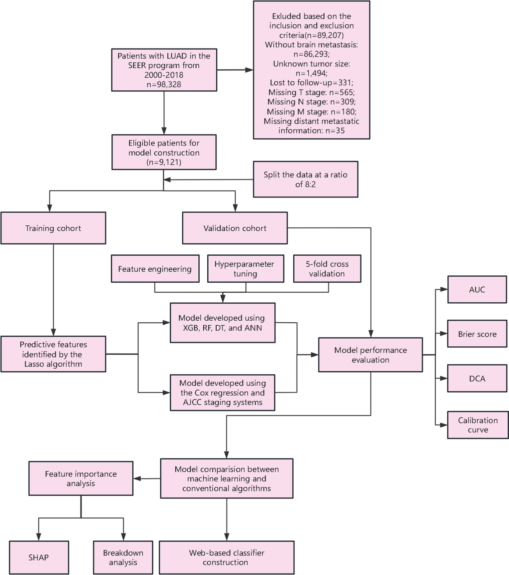
The criteria for inclusion in this study were as follows: (i) individuals diagnosed pathologically with LUAD between 2000 and 2018, classified according to the International Classification of Diseases for Oncology, third edition (ICD-O-3/WHO2008), with histopathological types specified by the ICD-O-3 His/Behave category for malignant neoplasms; (ii) patients presenting a single primary tumor without concurrent primary tumors at other sites; (iii) subjects confirmed to have BM at initial diagnosis. The exclusion criteria were: (i) missing demographic details such as age, gender, ethnicity, and marital status; (ii) incomplete clinicopathological information including histologic classification, precise primary tumor dimensions, tumor location and laterality, histological differentiation grade, metastases to bone, liver, or lungs, and TNM stage; (iii) lacking data on chemotherapy and radiotherapy treatments; and (iv) unavailability of survival status and follow-up information.

Data for this investigation were sourced from the SEER database, utilizing the SEER*Stata Software (version 8.4.0.1; https://seer.cancer.gov/data-software/).

2.3 Primary endpoint and baseline characteristics presentation

This study’s primary endpoint was OS, defined as the time from the date of cancer diagnosis to the date of death, regardless of cause. Baseline demographic and clinical features were systematically presented, with continuous variables summarized using means and standard deviations, and categorical variables described by frequencies and percentages. In total, 17 variables were examined to identify independent prognostic factors in patients with metastatic LUAD, which represented all the available parameters from the SEER database relevant to this population. Demographic parameters included age, sex, race, and marital status. Tumor clinicopathological characteristics featured histologic type, primary location, laterality, tumor grade (I, II, III, IV), tumor size, and the T, N, and M stages. Additionally, we assessed the presence of bone, lung, and liver metastases, as well as treatment details such as chemotherapy and radiotherapy.

2.4 Cohort division and data framework curation

To develop and validate the model, we systematically divided eligible patients into two cohorts: a training cohort and a validation cohort, using an 8:2 split generated by a stratified sampling approach. This stratification ensured that the proportion of patients with different prognoses was maintained in both datasets. Specifically, we utilized the initial_split() function from the rsample package in R and set a random seed for reproducibility. The training cohort was pivotal in creating the prognostic model and risk assessment classification system, playing a key role in the development of our analytical framework. Conversely, the validation cohort, separate from the training group, was essential for evaluating the model’s accuracy and ensuring the reliability of our findings. Within the context of machine learning, we optimized the classification threshold by employing a five fold cross-validation on the training cohort. This was aimed at enhancing the Area Under the Receiver Operating Characteristic Curve (AUC), a critical measure of the model’s predictive power.

2.5 Feature engineering and model construction strategy

For data preprocessing, prognostic categorical features were transformed using one-hot encoding, allowing for their seamless integration into our machine learning model. We first identified prognostic features influencing survival using the Lasso regression model. Based on these findings, we developed a Cox regression model to predict 1- and 2-year OS rates for LUAD patients with BM. Separately, we constructed a model using the AJCC staging system to provide an additional perspective on survival prediction. Furthermore, using the independent factors identified by Lasso, we applied four machine learning approaches: RF, XGB, DT, and ANN, with the mlr3 package in R, aiming to establish the most effective prognostic model for survival analysis.

RF, an ensemble learning method, improves predictive accuracy by aggregating multiple decision trees, each built from a random subset of the data and features, ensuring model diversity. To optimize RF performance, we tuned several key hyperparameters, including the number of trees (200 to 800), the minimum samples required for node splits (15 to 21), and the number of features considered per split (3 to 5), using grid search with a resolution of 10.

XGB, another advanced machine learning algorithm, enhances prediction accuracy by iteratively correcting errors from previous iterations. For XGB, we tuned the number of boosting rounds (nrounds, 100–200), the maximum tree depth (1–5), and the learning rate (eta, 1e−4 to 1), applying grid search with a resolution of 10 and five fold cross-validation to optimize performance.

DT provide an interpretable framework for survival analysis. We tuned two key hyperparameters for DT: the significance level (alpha), ranging from 0.01 to 0.1, and the minimum number of observations in terminal nodes (minbucket), set between 5 and 30. Grid search with a resolution of 10 was used for minbucket, alongside five fold cross-validation to evaluate model performance.

For the ANN, we employed the Adam optimizer and tuned key hyperparameters such as the learning rate (0–0.1), dropout rate (0–0.5), and weight decay (0–0.5). The network architecture was also optimized by adjusting the number of layers (1–3) and nodes per layer (5–13). To prevent overfitting, early stopping with a patience of 20 epochs and a validation fraction of 20% was used, with a maximum of 500 training epochs and a batch size of 32.

These comprehensive hyperparameter tuning strategies and model evaluations significantly contribute to advancing survival analysis for LUAD patients with BM, offering a robust and well-rounded approach to prognostic modeling.

2.6 Model performance evaluation

Model performance was assessed using several key metrics: time-dependent receiver operating characteristic (ROC) curve analysis, calibration curve analysis, decision curve analysis (DCA), and the Brier score. The model’s discriminatory ability was evaluated by measuring the AUC of the ROC curve, where a higher AUC value signifies greater accuracy in prediction. Calibration, a critical aspect of predictive modeling, examines how well the predicted probabilities match actual outcomes, aiming for a close fit to the 45° line in the calibration plot to indicate accurate predictions. DCA was employed to determine the model’s clinical utility, calculating net benefits across various threshold probabilities. Lastly, the Brier score, representing the mean squared difference between predicted probabilities and actual outcomes, was used to quantify prediction accuracy at specific time points, focusing on the concordance between predicted events (either survival or death) and observed results. The formula for the Brier score in survival analysis is given by:

$$Brier\,Score = 1/N\sum\nolimits_^ - O_ )^ }$$

A lower Brier score indicates better predictive accuracy, with a perfect score of zero representing a model that predicts events and non-events perfectly.

2.7 Model interpretation

We utilized the SHAP (SHapley Additive exPlanations) package to interpret machine learning models more transparently. Specifically, we made use of a summary plot provided by the SHAP framework to visualize how different variables contribute to the model’s predictions. Based on game theory, SHAP offers a structured approach to understanding the outputs of machine learning models. It enables the identification of key features that influence the model’s predictions and clarifies how these features affect the overall model output.

2.8 Statistical analysis

All statistical analyses were carried out using R software (version 4.2.1, https://www.r-project.org/). We applied two-tailed statistical tests, setting the significance level at p < 0.05 to determine statistical significance. The development of the model utilized a suite of R packages including “survival” for survival analysis, “mlr3verse” and “mlr3proba” for machine learning tasks, “mlr3extralearners” for additional machine learning algorithms, and “survex” for survival model extensions. For the interactive web-based model, we utilized the “shinydashboard” R package to create a dynamic interface.