AppendixAppendix I. Method for clustering of facilities2.1 Summary

The extent to which direct standardization can improve covariate balance is limited for facilities with small sample size, as is the case in our data. Specifically, in our facility data set, sample sizes per facility range from 1 to 45, with sample size smaller than 20 for 93% of the facilities. We address the issue of small sample sizes by clustering small facilities with similar facility characteristics into larger units of suitable size. Specifically, we grouped facilities into clusters with a sample of at least 40 clients, yielding a sample of 61 clusters of facilities. The characteristics of the resulting clusters, denoted \(_\), are a weighted average of the characteristics of the original facilities with weights proportional to the number of follow-up interviews in each facility in the cluster.

2.2 Approach

Notation: We denote by \(_\) the size of the sample of women from the fth facility, for \(f=1,\dots ,F\). For each facility, there is auxiliary information on a set of characteristics, \(_\in }^\), such as the type of facility (health center, health clinic, dispensary, pharmacy), whether the facility public, number of staff and indicators on services provided (antenatal, delivery, postnatal, postabortion, HIV related).

Clustering method: There are many ways in which facilities could be grouped to ensure a minimum sample size per cluster. We use a clustering algorithm to identify the grouping that maximize the internal homogeneity (Assunção et al. 2006), where homogeneity is defined in terms of the set of facility characteristics, \(_\), and a robust version of Mahalanobis distance (Rosenbaum 2010, sec 8.3).

Mahalanobis distance is a frequent used dissimilarity measure to summarize differences among multiple features while considering their correlation structure. Given the vector of characteristics, \(_\), the Mahalanobis distance between two facilities, f and f′, is defined as

$$ d_ }} = \sqrt - V_ }} } \right)^ \Sigma^ \left( - V_ }} } \right)} , $$

where Σ is the variance–covariance matrix of \(V\), the \(F\) by \(p\) matrix of facility characteristics.

While suitable for the multivariate Normal distribution, Mahalanobis distance can have poor performance with long-tailed distributions or rare binary covariates. Rosenbaum (2010) proposed a rank-based modification that avoids those shortcomings. The first part of the modification is to replace the entries of each of the variables, one at a time, by their relative ranking, with average ranks for ties. The second part of the modification is to pre-multiply and post-multiply the covariance matrix of the ranks by a diagonal matrix whose diagonal elements are the ratios of the standard deviation of untied ranks, to the standard deviations of the tied ranks of the covariates. Rosenbaum’s modified distance computes the Mahalanobis distance using the relative rankings and the adjusted covariance matrix.

The distance matrix can be further modified to emphasize particular variables using a penalty function. For example, for a particular characteristic \(w\), whenever \(\left| - w_}} } \right| > \zeta\), then \(d_}} \leftarrow d_}} + \beta\), with \(\upbeta \) some large quantity. This set-up favors near exact matching in the case of categorical variables (Zubizarreta et al. 2011).Footnote 3 We used this penalty with near exact matching on (i) facility type, (ii) whether the facility is a public facility, and (iii) the location, including the county and whether it a rural or urban setting.

Clustering algorithm: With a suitable measure of distance at hand we could, in principle, consider all assignments of facilities to clusters achieving a predefined minimum sample size per cluster, say\(_\), and chose the one assignment with the minimum within-cluster dissimilarity. Specifically, letting \(_\in \left\\) denote the cluster that the fth facility belongs to, we want to find \(_\) that minimize within-cluster dissimilarity, \(\frac\sum\nolimits_^ = k}} :C_}} = k}} }} } } }\), subject to \(\text\left(__=k}_\right\}}_^\right)\ge _\), considering all assignments, \(_\), over all possible total number of clusters, \(1<K<\text\).Footnote 4 In practice, an exhaustive search is unfeasible, and we need to use some iterative greedy algorithm to approximate the optimum. We used a minimum spanning tree (MST) based algorithm proposed by Assunção et al. (2006). MST algorithms are very fast and has been shown to have competitive performance (Gagolewski et al. 2023).Footnote 5

Once the clusters are found we extend the notation. We index the clusters by\(j=1,\dots ,J\), and use \(_\) to denote the size of the sample of women on the \(^\) cluster. We also have cluster characteristics, denoted by \(_\in }^\), constructed as weighted average of the characteristics of the original facilities, with weights proportional to each facility sample size, e.g., for the gth characteristic,\(_^=\frac_}__=\text}_^ _\). We subsequently refer to these clusters of facilities as either clusters or facilities interchangeably.

Appendix II. Weighting to produce standardized outcomes

In this appendix we provide additional details the estimation of the standardized measure of performance.

Recall that, for the each of the \(i=1,.., _\) women served in the \(^\) cluster of facilities have we observe a vector of background characteristics \(_\in }^\) such as age, marital status, or parity. We also observe an outcome, denoted by \(_^\), where superscript \(O\) indicates the specific outcome considered. In this study, \(O\in \\), where \(_^\) refers to the satisfaction score following the visit and \(_^\) refers to the binary indicator of contraceptive discontinuation at follow-up. The same superscripts are used to denote functions, models and model parameters that are specific to each outcome. Define \(_^\left(x\right)\equiv }(^|X=x, Z=j)\), the conditional expectation of the outcome in cluster j for a woman with a vector of characteristics x.

With this notation, the expected outcome in the jth cluster is given by \(_^=\frac_}__=j}_^\left(_\right)\), which we could easily be estimated with \( }_^=\frac_}__=j}_^}_\). This quantity, however, is not comparable across clusters. Even if a woman with the same set of characteristics, say x, would have the same expected outcome in cluster \(j\) or j′, i.e., even if \(_^\left(x\right)=_}^\left(x\right)\), the average outcome in the two clusters could differ because the distribution of covariates is not the same, i.e.,\(p\left(x|_=j\right)\ne p\left(x|_=\right)\). Thus, we are interested in the outcome we would have observed if the population served in all clusters was the same. While other target populations could be defined, we focus on the empirical distribution of the covariates across all facilities, i.e.,

$$_^=\frac__^\left(_\right).$$

3.1 Weighting

The primary estimator of the quantity of interest is a weighted average of observed outcomes for cluster j, using normalized weights \(}_\):

with \(\sum__=j}}_=1\). We want weights that make the covariate distribution of the two populations as similar as possible. Keele et al. (2021) proposed to use the weights that solve the following (convex) optimization problem,

$$ \mathop \limits_ \mathop \sum \limits_^ \left\^ - \mathop \sum \limits_ = j}} \gamma_ X_^ } \right\|^ + \lambda n_ \mathop \sum \limits_ = j}} \gamma_^ } \right\}, $$

subject to

where \( }^\equiv \frac_^_^\) and \(_^\) is some transformation of the original covariates \(_\) including standardization and feature expansion. Note that, while feature expansion is “optional” the standardization is necessary for the covariates to be given equivalent importance. The optimization problem trades off two competing terms for each facility j: better balance (and thus lower bias) and more homogeneous weights (and thus lower variance); with \(\lambda \) negotiating the tradeoff.

We constraint the weights to be non-negative (equivalently set \(=0\)) to avoid extrapolation, but do not set an upper limit. Figure 

Fig. 2

Covariate Balance vs. Variance Tradeoff as a Function of λ values. Each dot represents the average reduction in Mahalanobis distance (between the mean of the covariates in each cluster and the target population) and the average effective size for differ

2 display summaries measure of the tradeoff between covariate balance and variance for several values of \(\lambda \). Compared with no penalty at all, it appears that setting \(\lambda =0.001\) results on a substantial increase in effective sample size with very little cost in terms of increase imbalance; we selected that value for all the main analyses. As a sensitivity analysis, we also present the results for a choice of \(\lambda =0.1\) that discourage variation in the weights more aggressively (see sensitivity analyses).

Regarding \(^\), in addition to the main term for each individual level characteristics, we included indicators for thirdtiles for continuous variables (age, education, self-perceived wealth) to capture nonlinear relationships, and indictors for membership to some large segments based on marital status, age, and parity (i.e., single, between 15 and 25 years old, at most one kid; married, between 20 and 30 years old, at most two kids; married, more than 30 years old, three or more kids) to incorporate important interactions. All features were standardized (subtracted the mean and divided by standard deviation).

The resulting weighted estimator has the benefit of being design-based, i.e., the weights solving the optimization problem do not use any outcome information.

3.2 Variance estimation for the weighted estimators

This appendix presents additional detail on how we quantify uncertainty of the weighted and bias-corrected estimators. The approach to quantify uncertainty borrows from the field of survey sampling in which the use of weights has long tradition.

Recall we use \(_\) for the individual outcome (either discontinuity or satisfaction), \(_\) the binary indicator that individual \(i\) is in cluster \(j\), and \(}_\) are the weights that minimize the covariate between the sample in cluster \(j\) and a target population (the overall sample, in our case). Under the assumption that individual outcomes are sampled independently within facility, the sampling variance, conditional on the weights, is given by

$$ Var\left( _^W,O}} |\hat_ } \right) = Var\left( = j}} \hat_ Y_^ } \right) = \mathop \sum \limits_ = j}} \hat_^ Var\left( ^ } \right), $$

i.e., a weighted average of the individual-level variance in the outcome, \(Var\left(_^\right)\), which we will denote \(_^\right)}^\). For each facility, we could estimate the sampling variance (or its square root, the standard error) by plugging in an estimate of the outcome variance, say \(}_^\), i.e.,

$$ \widehat\left( _^W}} |\hat_ } \right) = \sqrt = j}} \hat_^ \left( ^ } \right)^ } = \hat_^ \sqrt = j}} \hat_^ } = \frac_^ }} = j}} \hat_^ } \right)^ }} = \frac_^ }}^ } }}, $$

where the effective sample size for facility j, is defined as \(_^\equiv \frac__=j }}_\right)}^}__=j }}_^}\), and, provided that \(__=j }}_=1\), simplifies to \(_^=\frac__=j }}_^}\) (Potthoff et al. 1992).

We could estimate the variance of the outcome by its sample counterpart, i.e.,

$$ \hat_^ = \sqrt = j}} \hat_^ }}\mathop \sum \limits_ = j}} \hat_^ \left( ^ - \hat_^W,O}} } \right)^ } . $$

This facility specific estimate, however, may be instable, particularly for facilities with small sample size. For example, in the case of discontinuity, it would be equal to zero in some facilities with no discontinuity events. For this reason, Keele et al. (2021) advocates for the use of a pooled estimate of the variance, a weighted average of the facility-specific estimates, with weights proportional to the effective sample size in each facility, i.e., \(}_^=\sqrt_^_^}_^_^}_^\right)}^}.\)

See also Bloom et al. (2017) for a discussion of this approach.

Appendix III. Comparison with other weighting strategies

For comparison purposes, we compute inverse probability of treatment weights (IPTW). ITPW are based on estimates of the (generalized) propensity score, i.e., \(_(x)\equiv \text\left(_=j|_=x\right)\), where \(_\) indicates the facility visited and \(_\) is the vector of covariates. The IPTW weights are given by

$$_^\equiv \frac__}\left(_\right)}.$$

We use the normalized version, \(_^}=\frac_^}__=_}_^}\). Because these weights can be quite variable, it is common practice to trim the weights at a given percentile \(q\), i.e., \(}_^=\text\left\_^,\text\left\^:q\le \widehat(^)\right\}\right\}\), before normalization.

As in Tang et al. (2020) we estimate the propensity score using multinomial logistic regression, i.e.,

$$}_\left(x\right)=\frac\left(_^_\right)}_^\text\left(_^_\right)},$$

with \(}_\left(x\right)=\frac_^\text\left(_^_\right)}\), the baseline category, and X includes a constant. It is common to truncate the weights. We consider weights truncated at several percentiles: 95% to 50% by 5% decrements. We present weights truncated at 95%, as representative of a typical choice, and 70%, because they maximize bias reduction over the grid considered.

As an alternative to multinomial logistic regression, we use a machine learning method to estimate the propensity scores, namely, gradient boosting (Friedman 2001). Gradient boosting algorithms approximate the conditional probability function by an ensemble of regression trees. As in other machine learning approaches, regularization could prevent extreme weights. We use the implementation by McCaffrey et al. (2013), which explicitly incorporates the balancing goal in the estimation, using balance measures as a criteria to select hyperparameters. We note that while this implementation of the algorithm was developed for more than two treatment levels, it is not optimized for the large number of “treatments” in a healthcare comparison setting as in our application.

Appendix IV. Performance “drivers” analysis

To identify facility characteristics that might predict differences in performance we examine the relation between our estimated standardized discontinuation rate, \(}_^\), and a set of facility-level characteristics,\(_\). This examination is carried out using regression. In the context of meta-analysis, the approach is termed meta-regression (Hartung et al. 2008, ch. 10), and it is used to examine factors driving effect heterogeneity across studies. Similarly, we use in the present context to identify predictors of differences in adjusted performance across clusters. As in the case of meta-regression, even if the input are valid causal estimates (from well conducted RCT), the regression only provides evidence of association.

Specifically, we hypothesize the following model for the standardized satisfaction in the jth cluster,

$$_^ |}_^\sim N\left(0,}_^}\right]}^\right),$$

$$_^| \tau \sim N\left(0, ^\right]}^\right),$$

where \(\delta \) is a vector of regression coefficients, relating adjusted performance with the facility level characteristics linearly, \(_\) represents variation of performance across clusters not explained by those characteristics, and \(_\) is the sampling error (the error arising from the observing only a sample of women served in facilities in that cluster). As it is common in meta-analysis or small area estimation (in that context, this model is known as Fey-Harriot) we take the first level variation (i.e., \(}_\)) as a known quantity (its estimation is discussed in Appendix II). The normal distribution for the error can be justified in terms of the expected distribution of the estimator of standardized performance (i.e. a weighted average) on large samples.

In the case of discontinuation, we start by defining the “effective number of cases” (as in Chen et al. 2014), \(}_^\equiv _^\times }_^.\) We can then model the effective count as

$$}_^ \sim \mathito\mathit\left(_^, _^\right) ,$$

$$_^=}^\left(_^+_^^\right),$$

$$_^| ^\sim N\left(0, ^\right]}^\right) ,$$

Note that we use a different superscript for the standard deviation across facilities, \(^\), which is in different scale that \(^\).

Importantly, with both these models we posit an underlying distribution for the unexplained variation of standardize performance across facilities. The introduction of this random effect induces some extent of pooling across individual estimates of standardized outcomes, particularly when the estimates are more uncertain (e.g., clusters with small effective sample size).

The models are completed with weakly informative prior for the variance across facilities, we use for both outcomes a half student-t with 3 degrees of freedom and a scale parameter of 2.5, i.e., \(p(\tau )\propto \right)}^\right)}^}\) with \(\left(\upsilon ,A\right)=(3, 2.5)\) (Gelman 2006) and flat, improper prior distributions for the vector of regression coefficients, i.e., \(p\left(\delta \right)\propto 1\). Given the data (i.e., the bias-adjusted estimates taken as data), draws from the posterior distribution were obtained via MCMC. We use the R package brms (Bürkner 2017) to interface with stan (Stan Development Team 2021). We used conventional diagnostics, such as \(\widehat\) and effective sample size, to check MCMC convergence.

Appendix V. A comparison with model-based approach to standardization

We compare the results from our analysis from those that would have been obtained from a more conventional, model-based approach to standardization.

An alternative approach to estimate adjusted performance is to model the outcome directly from the start using a hierarchical model. This approach is frequently used as the basis of so called “indirect standardization”. For example, for a binomial outcome, such as contraceptive discontinuation, the likelihood for the outcome would be given by

$$_^ | _^ \sim Bernoulli\left(}^\left(_^\right) \right),$$

$$_^|_^, _^ \sim N\left(_^,_^\right]}^ \right),$$

In turn the satisfaction outcome,

$$_^| _^,\sigma \sim N\left(_^, _^\right),$$

$$_^|_^, _^ \sim N\left(_^,_^\right]}^ \right),$$

where (\(^,^\)) and (\(^,^\)), are vectors of regression coefficients. Bayesian estimation of this model requires prior for all the parameters; flat priors for (\(^,^\)) and (\(^,^\)), for variance parameters, \(_^\), \(_^\), and \(_^\).

The \(\vartheta \)’s can be interpreted as an adjusted measure of performance (in the case of a binary outcome, in a logistic scale); for example, if the vector of individual level characteristics, \(_\), is centered at their grand mean, then \(_\) would be the expected value of that measure in the \(^\) facility for a woman with “average characteristics”. Consequently, the \(\zeta \)’s (as the \(\delta s\) in our main approach) capture systematic difference in this measure of adjusted performance associated with facility-level characteristics.

While not a customary for indirect standardization,Footnote 6 we can obtain model-based estimates of our quantities of interest (Varewyck et al. 2014). These are given by,

$$ \hat_^H,D}} = \frac\mathop \sum \limits_^ }^ \left( _^ \left( ,W_ } \right)} \right), $$

And

$$ \hat_^H,S}} = \frac\mathop \sum \limits_^ \hat_^ \left( ,W_ } \right), $$

where we use the superscript H, to distinguish these estimates from our weighted (W) alternative. These quantities are computed on each posterior sample from \(}_^|^\) and \(}_^|^\), respectively, from which we can summarize uncertainty.

6.1 Average predictive difference

We can further compare the predictive impact of facility-characteristics implied by this model vis-à-vis the one implied by our proposed approach (see for example, Gelman and Pardoe (2007) for a similar approach). For a given facility-level characteristic, say \(u\in W\), we select a pair of values \(\left(^,^\right)\), such as its 2.5% and 97.5% percentiles, and compute the quantity of interest again, altering only that input.

$$ PD_^ = \frac\mathop \sum \limits_^ \hat_^O,M}} \left( ,W_^ }} } \right) - \frac\mathop \sum \limits_^ \hat_^O,M}} \left( ,W_^ }} } \right), $$

where the superscript \(O=\\) stands for outcome (i.e., either satisfaction or discontinuity) and \(M=\\) signals the type of estimator (e.g., based on the standardized outcome or on hierarchical regression).

The measure \(P_^=\frac_P_^\), the predictive difference average over the facilities, is directly comparable across approaches.

6.2 Simulation set up

To compare direct standardization with balancing weights with more conventional hierarchical regression modeling we implement a simulation.

The simulated data is designed to resemble discontinuation in the real application. We first construct a large population (\(N=\text\)), and then sample repeatedly from this population for each of the \(J=61\) facilities, \(_\) cases per facility, where \(_\) is as in the real application.

Each case in the population is characterized by three binary covariates, each drawn from a Bernoulli distribution, i.e., \(_ \sim Bernoulli(.5)\) for \(k=1, 2, 3\), and J potential outcomes, \(_(j)\), drawn from

$$_^(j) | _ \sim Bernoulli\left(\Phi \left(_\right) \right).$$

In each of three scenarios, we set \(_\) so that the estimand  \(_^=\frac_^\Phi \left(_\right)\) is approximately equal to \(}_^\), the standardized discontinuity estimated in the real application (this is achieved by group centering \(_\) and adding \(^\left(}_^\right)\)). In all scenarios, we sample repeatedly from this population, with probability proportional to “size”, where the measure of size depends on \(_\) and the facility, to ensure unequal distribution. Specifically, we set \(s_ = Unif\left( \left( } \right)} \right) + Unif\); in half the facilities the probability of selection is proportional to \(_\) while in the other half, the probability is proportional to \(1/_\). In each sample, we set the observe outcome to\(_=_^(_)\). The three scenarios differ in the following way:

Scenario 1: No confounders

where \(_\) is a facility-specific intercept, set equal to \(^\left(}_^\right)\) in this scenario.

Scenario 2: A confounder, \(_\), with homogenous effect

Scenario 3: A confounder, \(_\), which affects the outcome differently, depending on the facility

$$ \eta_ = \vartheta_ + X_ \cdot 1\left( \le 30} \right) - X_ \cdot 1\left( > 30} \right) $$

To summarize the performance of the different estimators we use the following measures. Let \(}}^\) denote the \(J\)-dimension vector of true values, and \(}}}^\) the estimator vector. We define the root mean square error as,

$$RMSE\left(}}}^\right)\equiv E\left(^\left(}}}^-}}^\right)\Vert }_ \right)=E\left(\sqrt_}_^-_^\right)}^}\right) ,$$

and the mean absolute error as,

$$MAE\left(}}}^\right)\equiv E\left(^\left(}}}^-}}^\right)\Vert }_\right)=E\left(\frac _\left|}_^-_^\right|\right).$$

Let \(}}}_^\) and \(}}}_^\) be the vectors of lower and upper limits of the 95% confidence or credible intervals around \(}}}^\). We define the 95% CI Coverage as,

$$Coverag_(}}}_^,}}}_^) \equiv E\left(\frac_1\left(}_^\le _^\le }_^\right)\right),$$

where \(1(.)\) is the indicator function. These expectations are estimated with the average over 200 replications. For example, \(\widehat\left(}}}^\right)=\frac_^\left(}}}^-}}^\right)\Vert }_\), where \(}}}^\) is the value of the estimator vector in the \(^\) replication, and\(R=200\).

Appendix VI. Sensitivity analyses

In this appendix, we present result after altering the balancing weights by increasing the penalty for dispersion.

Altering the choice of penalty to obtain balancing weights.

Recall that the penalty parameter, \(\lambda \), regulates the tradeoff between precision (measured for example by the effective sample size) and covariate imbalance (and consequent bias). Since different choices are possible, we rerun the analysis by selecting a different value for lambda, \(\lambda =.1\), which penalizes dispersion more aggressively.

Results based on the new set of weights are presented in Table 

Table 6 Imbalance and bias reduction and effective sample size after weighting

6. As we penalized the weight variability more, the weights can remove less imbalance. Nevertheless, the results are pretty much unaltered. See Table 

Table 7 Comparison of average predictive difference (APD) using set of weights based on different values for the penalty parameter

7

Appendix VII. Supplementary tables

See Table 

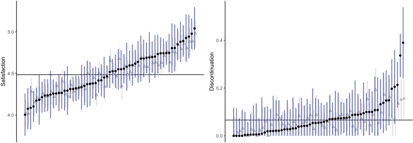
Table 8 Facility characteristics reference

8

Appendix VIII. Supplementary figures

See Figs.

Fig. 3

Boxplots of mean outcomes per cluster before and after weighting. Red line represents the marginal mean, i.e., the average outcome for all women combined

3,

Fig. 4

Residual imbalance after weighting by size. Imbalance is measured with average Mahalanobis distance (\(_^\)) discussed in Appendix II

4 and

Fig. 5

Unadjusted vs. weighted discontinuation

5