Study population

Data for the study came from two prospective longitudinal population cohort studies, the BC Generations Project (BCGP) and Alberta’s Tomorrow Project (ATP). BCGP consists of 29,788 participants from across British Columbia, aged 35 to 69 at time of recruitment, which occurred between 2009 and 2016 [15]. ATP consists of 54,922 participants from across Alberta, aged 35 to 69 at time of recruitment, which occurred in two phases (Phase I, 2000–2008; Phase II, 2009–2015) [16]. During Phase II, newly recruited participants and a portion of previously recruited participants (n = 24,075) completed questionnaires similar to those completed by BCGP participants at time of recruitment. These questionnaires collected health and reproductive history, social demographic characteristics, and behavioral factors. As both BCGP and ATP belong to the Canadian Partnership for Tomorrow’s Health (CanPath) [17], these questionnaires underwent an extensive harmonization process. Participants also provided height and weight measurements either via in-person assessments at a study center or through self-report. Participants provided blood samples, which were divided into aliquots of plasma, serum, buffy coat, and red blood cells and stored at -80 °C.

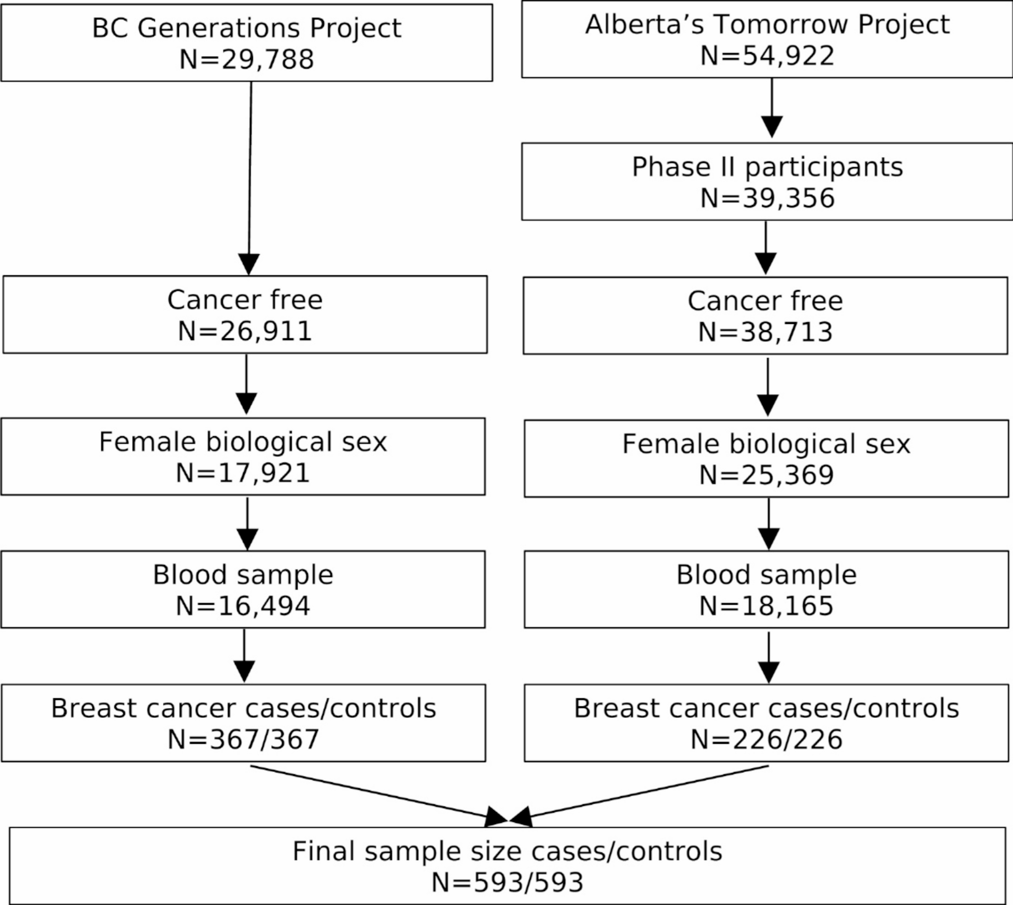
Study design

Participants were eligible to be included in the current study if they were female, completed a questionnaire (baseline questionnaire for BCGP; Phase II questionnaire for ATP), provided blood samples at time of questionnaire completion, and were cancer-free, except for nonmelanoma skin cancer, at time of questionnaire completion (Fig. 1). A total of 16,494 BCGP and 18,165 ATP participants met these eligibility criteria. Among these participants, cases were selected if they were diagnosed with incident invasive breast cancer. Incident invasive breast cancer cases were identified through annual linkage with each province’s respective Cancer Registry (International Classification of Diseases for Oncology, Third Edition site code: C50.x; morphology codes: 80103, 80323, 80413, 81403, 82003, 82113, 82553, 84013, 84803, 85003, 85033, 85043, 85073, 85203, 85223, 85233, 85243, 85403, 84413, 85753, 89833). Based on morphology codes, cases were classified into four histological subgroups: invasive ductal (85003, 85043, 85073), lobular (85203), mixed ductal/lobular (8522, 8523, 8524, 8255), and other carcinomas. In addition, cases with known hormone receptor expression status were categorized as: luminal A [estrogen receptor positive (ER+) and/or progesterone receptor positive (PR+) and human epidermal growth factor receptor 2 negative (HER2-)], HER2+, and triple-negative breast cancers.

Fig. 1

Inclusion criteria for study of serum metabolome and breast cancer risk

Each case was matched to a single control who was cancer free at the time of case diagnosis, except for nonmelanoma skin cancer, on source cohort, baseline menopause status, age at blood collection (± 2 years), and year of blood collection. Those with missing menopause status (n = 16) were classified as premenopausal if age at time of questionnaire completion was under 51 and postmenopausal if age at time of questionnaire completion was 51 – the median age at natural menopause reported in Canada – or older [18].

Health, lifestyle, and reproductive data

Body mass index (BMI), measured in kg/m2, was calculated based on height and weight data collected during in-person assessments (80% of eligible participants). For those without in-person height and weight data, self-reported measures from the harmonized questionnaire were utilized. Other factors obtained from the questionnaire included age at time of questionnaire completion (same as age at blood collection), ethnicity, annual household income, highest attained education, family history of breast cancer (first degree relatives), age at menarche, number of live births, age at first pregnancy, history of oral contraceptive use, history of hormone replacement therapy, alcohol consumption (average over last year), and smoking status. Missing covariate data were assumed to be missing at random and, as such, were imputed using the Multiple Imputation by Chained Equations (MICE) algorithm [19]. All risk factors and the outcome were used as auxiliary variables for imputation. Ten imputed datasets were generated, each with thirty iterations [20].

Metabolomics data

Non-fasting serum samples (30 µl each) were plated on 96-well plates and shipped to General Metabolics LLC (Boston, Massachusetts). For a randomly selected 5% of participants, an additional sample was included as a blind duplicate for quality control assessment. Metabolites were measured using previously described MS methods [21]. Briefly, each sample was diluted with 180 µl of 80% ethanol in water. 5 µl of the resulting solution was injected twice, consecutively, at a flow rate of 0.150 ml/minute, into an Agilent 6550 iFunnel Quadrupole time-of-flight (Q-TOF) mass spectrometer. Blanks, pooled study samples, and National Institute of Standards and Technology standard reference materials were injected after every 48 study samples for quality assurance. Metabolites were detected as peaks with specific mass-to-charge ratios (m/z), and the intensity of each peak was a measure of the relative abundance of each metabolite. All peaks with m/z between 50 and 1,000 were recorded for each sample. For those samples with missing values for a particular metabolite (i.e., no peak detected in the sample), the missing values were backfilled using the measured intensity in the sample at the recorded m/z for that metabolite.

Mass spectra data were processed by General Metabolics using MATLAB (The Mathworks, Natick, MA, USA). Metabolite annotations were identified by comparing measured m/z to theoretical m/z within 0.001 Da recorded in the Human Metabolome Database (HMDB) and the Kyoto Encyclopedia of Genes and Genomes (KEGG) database and cross-referenced against the Chemical Entities of Biological Interest (ChEBI) database [22,23,24]. Since no chromatographic separation was performed in tandem with mass spectrometry, it was not possible to distinguish between metabolites with identical molecular formulas.

Metabolites that were missing in over 50% of the study samples were excluded. Coefficients of variation (CVs) were calculated to assess reproducibility based on the blind duplicate samples. For each pair of duplicate samples, the CV of each metabolite was computed by dividing the standard deviation (SD) by the mean ion intensity, and median CVs across all samples were calculated. Metabolites with median CVs above 20% were excluded. Metabolite intensity measures were normalized using a cubic spline method [25].

After normalization, duplicate intensity measures for each metabolite were averaged to obtain a single measurement per participant. To account for the matched study design, the mean intensity measure of each metabolite in a matched pair was set to zero [26]. In addition, each metabolite intensity was divided by the standard deviation across all samples to assess breast cancer risk associated with one standard deviation increase in metabolite intensity.

Statistical analysis

Associations of each metabolite with breast cancer risk were estimated using unconditional logistic regression adjusted for matching factors [source cohort (BCGP or ATP), menopause status (pre- or post-), age at blood collection (continuous), year of blood collection (2009–2019, 2011–2012, or ≥ 2013)] (R version 4.3.2). Multiple testing was accounted for by applying the Benjamini-Hochberg procedure with the false discovery rate (FDR, also known as q-value) set at 0.1. For metabolites that were deemed significant after multiple testing correction, we fitted separate logistic regression models to investigate the potential for confounding effects by established breast cancer risk factors, including ethnicity (White or Non-white), annual household income (<$50,000, $50,000-<$100,000, or ≥$100,000), highest attained education (high school or less, some post-secondary, or Bachelor’s or higher), family history of breast cancer (yes or no), age at menarche (< 12 years, 12–13 years, or ≥ 14 years), number of live births (continuous), age at first pregnancy (never pregnant, < 25 years, 25–29 years, or ≥ 30 years), oral contraceptive use (ever or never), hormone replacement therapy (ever or never), BMI (< 18.5–24.9 kg/m2, 25.0–29.9 kg/m2, or ≥ 30 kg/m2), alcohol consumption (none, 1–3 times/month, 1–3 times/week, or ≥ 4 times/week), and smoking status (never, past, or current). Analyses were completed on each of the imputed data sets and the resulting odds ratio (OR) estimates were averaged. A pooled Wald-based 95% CI was generated using Rubin’s Rule [27]. Statistically significant metabolites from the overall analysis were also evaluated in the following subgroups: participants who were postmenopausal at time of blood sample collection, cases diagnosed with invasive ductal carcinomas along with their matched controls, and cases diagnosed with luminal A breast cancers and their matched controls. Numbers of other breast cancer subtypes were insufficient to conduct meaningful analyses.

Risk prediction models were developed using partial least squares discrimination analysis (PSL-DA) (R version 4.3.2) [28]. Prediction models were generated using the metabolites found to be statistically significantly associated with breast cancer in the overall logistic regression analysis, with and without established breast cancer risk factors (all models included matching factors). For each model, 80% of the data were used as a training set and 20% were used as a testing set. Pair identifiers were used to split the data to preserve the matched design. For cross-validation, training data were randomly split into 10 equal-sized subsets, each also maintaining case-control matching. Nine subsets were used to train the algorithms across a grid of hyperparameters, and the tenth subset was used to test performance. This process was repeated 10 times, and the hyperparameters that resulted in the highest cross-validated area under the curve (AUC) were used to predict outcome in the testing data set. One-hundred models were generated from 100 independent training-testing partitions. The empirical mean and 95% CI for predictive performance were calculated.