We present an experimental setup for automated data acquisition of needle punctures using a robot. US volumes of needle insertions are acquired in water as an imaging medium as well as in chicken liver tissue. We perform needle insertions parallel to the ultrasound coordinate system and at tilted angles. For needle tip detection, we propose a deep learning approach and compare its performance with a conventional segmentation approach.

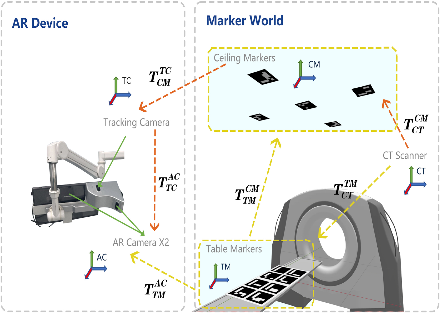
An overview of our experimental setup for data acquisition is depicted in Fig. 1. Our setup contains a hexapod robot, a US system with a custom volumetric US probe and a needle. The needle has a trocar needle tip and a diameter of 2.15 mm. The hexapod (Hexapod H-820, PI, DE) with axial repeatability of 20 \(\upmu \)m drives the needle relative to the volumetric US probe which is rigidly mounted to a base plate. The US probe (Vermon, FR) contains 16 \(\times \) 16 elements embedded at a pitch of 0.3 mm and has a central frequency of 3 MHz. Volumetric image data are acquired with a 256-channel US system (Griffin, Cephasonics, USA) by connecting each element to an individual channel without multiplexing.

The transformation matrices and notations of our setup are depicted in Fig. 1a. First, the transformation between hexapod base (H) and needle tip (NT) in the hexapod coordinate system (\(^}}T_}}\)) is estimated with a hand-eye-calibration and the QR24 algorithm [4]. For needle calibration, we use external markers attached to the needle shaft and a tracking camera (fusionTrack 500, Atracsys, CH) with a resolution of 0.09 mm and a temporal sampling rate of 200 Hz. We report a translational error of 0.07 mm and a rotational error of \(^\) based on 761 different poses of the robot. Second, we estimate the transformation from hexapod (H) to US (US) coordinate system (\(^}}T_}}\)), assuming parallel coordinate axes and a pure translational transformation. We determine the needle tip position in acquired US volumes using conventional image processing methods. The translation offset between the US and hexapod coordinate systems is calculated by minimizing the mean error between the detected needle tip positions in the US volume and the corresponding hexapod poses. Please note that the needle tip ground truth positions in the hexapod coordinate system are given in mm; hence, we divide them by the pixel resolution of 0.3 mm to get the hexapod pose in pixel units.

We use the open-source framework SUPRA [6] to acquire focused B-Mode US volumes with a sampling frequency of 4Hz, an imaging depth of 5mm to 40mm, and an opening angle of \(^\). We apply beamforming and construct our US volumes from 16 beams while assuming a constant speed of sound of 1500 m/s. This results in US volumes of 117 \(\times \) 134 \(\times \) 134 pixels along the depth and lateral axes, respectively. Assuming a pixel resolution of 0.3 mm in all dimensions we report an effective field of view (FOV) of 5–40mm along the depth axis and a maximum lateral width of 40.35mm. We track the needle movement with a temporal sampling rate of 200 Hz by recording the hexapod positions.

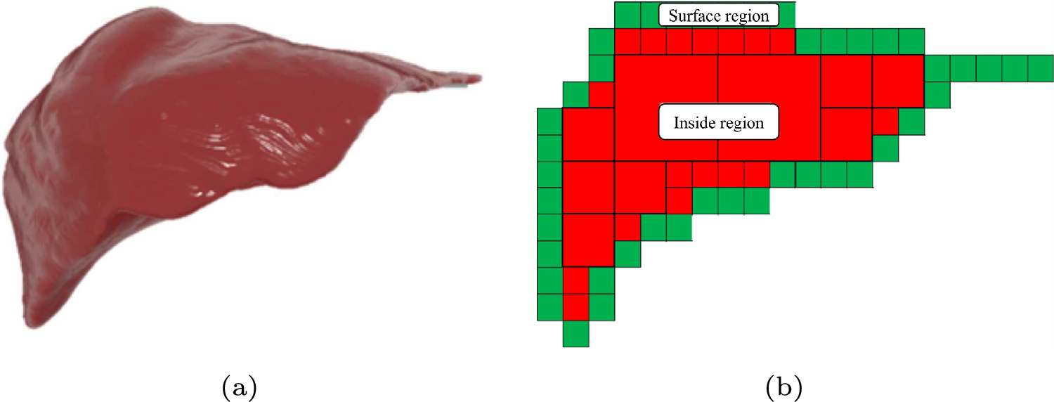
We perform needle insertions in water as well as in chicken liver tissue. We manufacture a phantom with a fresh chicken liver embedded in 10% gelatine concentration. To enhance speckle, we add graphite powder to the gelatine before pouring. The phantom is depicted in Fig. 1b. Exemplary low-resolution US volumes of needle insertions acquired in water and liver are shown in Fig. 2. The needle is inserted in \(y_\text \)-direction over a distance of 15 mm. During needle insertion, we constantly acquire US volumes and track the needle movement based on the hexapod position.

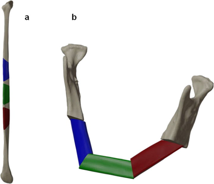
First, we perform twelve needle insertions parallel to the \(y_\text \)-direction of the US coordinate system. Based on the orientation of the setup components shown in Fig. 1a, we assume that the needle moves in the negative \(y_\text \)-direction of the US coordinate system with a velocity of 1.5 mm/s. In Fig. 3, the driven needle trajectories are shown in the hexapod coordinate system. The insertions are performed at different starting positions relative to the US volume by varying the needle height \(z_\mathrm}\) ([−8, −10, −13, −18] mm) and horizontal \(x_\mathrm}\) position ([−15, −20, −25] mm). In total, our data set with the needle aligned parallel to the US coordinate system contains about 600 US volumes acquired in water and another 600 volumes in liver tissue.

Second, we investigate the feasibility of tracking the needle tip while the needle axis is tilted, hence not aligned to the US axis. We perform needle insertions with the needle rotated around the \(x_\mathrm}\) axis (\(\alpha _}}\)) and \(z_\mathrm}\) axis (\(\alpha _}}\)). We use three different needle angles (\(\alpha _}}=\pm 5^\), \(\alpha _}}=-5^\)) in water. For each needle angle we perform nine insertions with a velocity of 1 mm/s in needle axis direction with different \(x_\mathrm}\) and \(z_\mathrm}\) positions. Our tilted data set contains about 2000 US volumes acquired in water.

Trajectory showing the acquired needle positions in water and liver in hexapod coordinates. The colors indicate exemplarily for fold 1 whether data are used for training, validation, or testing. Needle insertion is performed along positive \(y_}}\) direction. Note that we can differ between a test set at medium and bottom depth

We use a 3D DenseNet architecture to directly predict the 3D needle tip position from a US volume as input. Our network is based on a DenseNet-121 architecture [7] while we extend the data processing to three dimensions. For efficient training, we crop the US volume to a FOV of 11.25–40 mm along depth direction and 7.5–32.85 mm in \(x_}}\)- and \(y_}}\)-direction. Please note that we only crop the US volumes and do not perform any additional pre-processing. We define a regression problem to receive the three-dimensional position vector of the needle tip as the output of the network. All US volumes are fed into the network with labels describing the 3D position of the needle tip. We distinguish between experiments where we use the recorded needle tip positions in hexapod coordinates (\(\text _\text \)) as the training target and the positions in US coordinates (\(\text _\text \)) as the training target. For our quantitative analysis we use the hexapod coordinates as training target as they are more precise and eliminate additional inaccuracies due to US image distortions in the calibration between ultrasound and hexapod. All networks are trained for 800 epochs with a batch size of 8, a learning rate of \(}}\), using the Adam optimizer [8]. We define the loss function as the mean squared error between the label and the predicted vector of the needle position. For testing, we use the model which shows best performance on the validation data set.

For our experiments with the needle axis parallel to the US coordinate axis, we train two individual networks on US data acquired either in water or from the liver phantom. For each network, we perform a fivefold cross-validation on the twelve insertion data sets acquired. For each fold, we define two insertion paths for testing, two insertion paths for validation, and the remaining ones for training. The test data set remains the same for all five folds. For the test data, we use an insertion path positioned at a medium depth and one positioned at a lower depth of the US volume, hereafter referred to as the upper and bottom test set, respectively. For the validation data set, we use a new pair of insertion paths for each fold. We make sure these two paths do not lie in the same plane along the \(z_}\)-axis or \(x_}\)-axis. Figure 3 shows the respective data split for fold 1.

For the data set with tilted needle axis, we perform a fivefold cross-validation on the nine insertion data sets acquired. For each fold, we randomly define three insertion paths for testing (one path per needle angle), six for validation (two paths per needle angle), and the remaining ones for training.

The trainings are performed on a NVIDIA GeForce RTX 4090 GPU.

The main steps of the conventional segmentation approach (CSM) for needle tip detection are shown in Fig. 4. First, we identify the region of interest (ROI) containing the needle. For this, we assume that the needle is the largest structure in the US image. We apply a median filter (size=[25, 3, 3]) and search for the largest contiguous area with pixel values greater than 128 in the US image. We define a ROI that is centered in the largest structure with ± 25 pixels in the \(x_\text \)- and \(z_\text \)-direction. The \(y_\text \)-direction is not cropped. In the next step, the needle is segmented in the original US image, cropped to the ROI and its needle tip is detected. We perform a binary image segmentation based on a fast marching method using weights based on weighted grayscale differences. We define the needle tip as the farthest point from the edge of the segmented structure.

Conventional needle tip tracking: main steps of the conventional segmentation method for needle tip tracking. First, a ROI is defined. Second, the needle is segmented and the needle tip is computed. The volumes are visualized using maximum intensity projection and the jet colormap

In our conducted experiments, we mainly differ between the chosen method for needle tip detection and the medium in which we perform the insertions. First, we evaluate the tracking performance of our conventional segmentation approach compared to our deep learning approach. For this analysis, we use the parallel needle insertion data in water only. Second, we compare the needle tip prediction performance when using the hexapod position as training label compared to using training labels in the US coordinate system. Third we evaluate the performance on a liver data set. In the end, we evaluate the performance on a data set with tilted needle orientations. We evaluate the needle tracking performance of the different experiments based on the mean absolute translation error

$$\begin e(x_\mathrm}, y_\mathrm}, z_\mathrm}) = \sum _^|l_i-p_i| \end$$

(1)

over N US volumes with \(l_i\) denoting the training label and \(p_i\) the predicted target position.