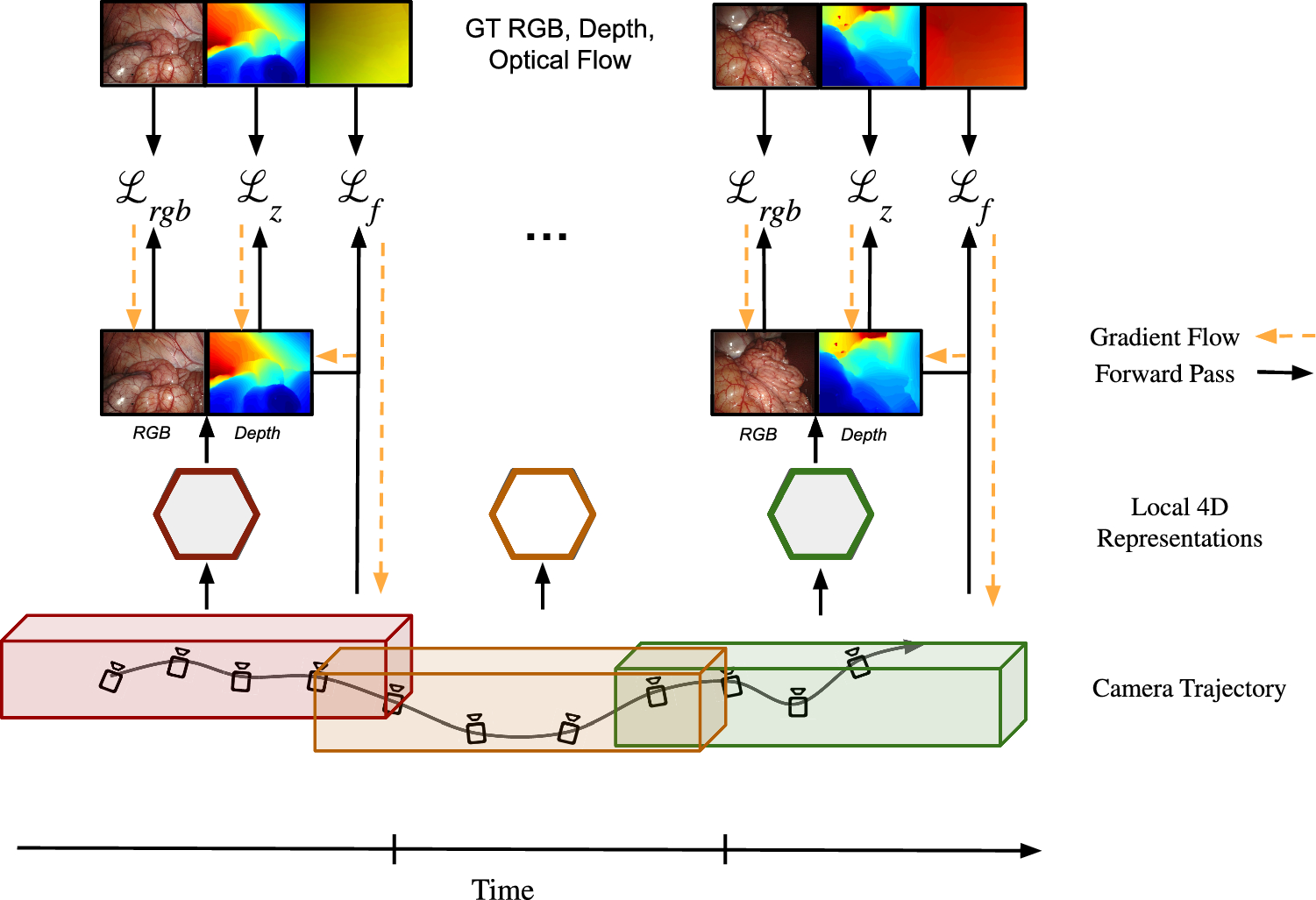
Given a rectified stereo endoscopic video, our goal is to reconstruct the 4D scene accurately without prior camera pose information. For this, we propose a new method FLex, standing for Flow-optimized Local Hexplanes, depicted in Fig. 1, which combines advancements from recent NeRF literature to build multiple smaller dynamic models that are progressively optimized. In contrast to prior work [7, 8, 10], we do not have one unified representation of the scene but multiple smaller overlapping ones. The representation of local models allows us to represent boundlessly large scenes, both temporally and spatially, accurately without incurring prohibitive memory growth while maintaining a high feature grid resolution. Furthermore, adopting a progressive optimization scheme enables the optimization of poses from scratch. Since endoscopic environments often have textureless surfaces which make geometry optimization from photometric consistency difficult we additionally incorporate supervision through optical flow and stereo depth priors.

NeRFs [6] implicitly model a 3D scene utilizing differentiable volume rendering to predict pixel colors. They can be adapted to a 4D scene representation by adding the timestep k as an additional input to the model. The color \(\hat(\textbf)\) of a ray \(\textbf=\textbf+\textbft\) with origin \(\textbf\) and direction \(\textbf\) at timestep k is calculated from the density \(\sigma \) and color c that are output from the model with volume rendering:

$$\begin \hat(\textbf) = \int _^ w(t) \cdot c(t) \textbft, w(t) = \exp \left( -\int _^ \sigma (s) ds \right) \cdot \sigma (t). \end$$

(1)

Using these rendering weights w, the expected termination depth \(\hat\) of the ray \(\textbf\) can be calculated by taking the weighted sum of each sampling location t along the ray between \([t_,t_]\).

$$\begin \hat = \int _^ w(t) \cdot t\ \textbft \end$$

(2)

The continuous integral in Eqs. (1), (2) is discretized following [6]. We choose HexPlane [24] as our local model, which represents a dynamic scene using an explicit 4D feature grid paired with an implicit MLP. The grid is constructed from several planes, where each plane represents a combination of two dimensions, three spatial dimensions and one temporal dimension, yielding six planes in total. During ray-casting, the corresponding features on each plane are extracted for the spatio-temporal sampling locations along the ray and combined by multiplication and concatenation before being fed into smaller MLPs and similarly to NeRF [6] rendered with volumetric rendering. For more details regarding HexPlanes [24] architecture we refer the reader to the original publication.

Endoscopic videos contain two main challenges for NeRF architectures: They are dependent on external tools for accurate pose estimation and can constitute arbitrarily long sequences of a dynamic environment. In order to tackle these two problems in a robust and efficient way, our joint pose and radiance fields optimization scheme combines the concepts of progressive optimization and dynamic allocation of local HexPlane models as visualized in Fig. 1 and inspired by LocalRF [18].

In the scope of progressive optimization, we start with the first five frames of the sequence, in which the first frame of the video is assigned an identity pose matrix, then we consecutively add one frame at a time, initializing its camera pose parameters with the previous frame’s camera pose. When the appended frame increases the number of frames above a preset threshold, \(t_\), or the distance between the optimized position of the camera and the center of the current local model is larger than a distance threshold, \(t_d\), we instantiate a new local model, setting this new frame to be its origin. To ensure consistency across local models, we assign the last thirty frames of the previous model to be overlapping with the new local model. To secure a coherent trajectory during progressive optimization, we consistently sample rays from the last four appended frames. During inference, if a pose corresponds to the spatial and temporal extent of multiple local models, each model’s contribution is aggregated into the ray-casting formulation with blending weights linearly set on the overlapping regions based on the proximity to the centers of the local models. Before a new local model is initialized, the last model goes into a refinement phase where the pose and model parameters are optimized with batches of samples uniformly picked along its entire span.

We employ the common photometric loss \(\mathcal _\) as defined in Eq. (3) with ground-truth \(C(\textbf)\) and predicted \(\hat(\textbf)\) pixel values for ray \(\textbf\) within the set of rays \(\mathcal \):

$$\begin \mathcal _ = \frac|}\sum _\in \mathcal }\left\| \hat(\textbf) - C(\textbf)\right\| _^ \end$$

(3)

We also employ geometric regularizers by applying a depth supervision loss along with line-of-sight priors as introduced by Rematas et al. [25]. We denote them together as \(\mathcal _\), composed as \(\mathcal _ := \mathcal _\textrm + \mathcal _\textrm + \mathcal _\textrm\).

For the depth loss, the predicted depth \(\hat\) for ray \(\textbf\) is optimized with the ground-truth depth z via an L2 loss:

$$\begin \mathcal _\textrm = \frac|}\sum _\in \mathcal }\Vert \hat(\textbf)-z(\textbf)\Vert _^ \end$$

(4)

The line-of-sight priors regularize the density values along a ray to be concentrated on the actual surface, thereby, together with the depth loss, improving the capture of the scene geometry. Given a set of data samples D, \(\mathcal _\textrm\) ensures that the rendering weights w(t) around the region of z follow a Gaussian distribution, where \(\mathcal _(x) = \mathcal (0, (\epsilon /3)^2)\) (see Eq. (5)). \(\epsilon \) is initially set to be 1 cm and, over time, exponentially reduced to 1 mm.

$$\begin \mathcal _\textrm = \mathbb _ \sim \mathcal } \left[ \int _)-\epsilon }^)+\epsilon } \left( w(t) - \mathcal _(t-z(\textbf))\right) ^2 dt \right] \end$$

(5)

Additionally, a penalty is added for the rendering weights w(t) in the empty region to push them toward zero, as depicted in Eq. (6). The empty region is defined from the nearest sampling point \(t_\) until the surface region is covered in Eq. (5).

$$\begin \mathcal _\textrm = \mathbb _ \sim \mathcal } \left[ \int _}^)-\epsilon } \left( w(t)\right) ^2 dt \right] \end$$

(6)

One of the main strengths of our method during the initial phase of our progressive optimization is the supervision via an optical flow loss \(\mathcal _\) in both temporal directions as described in Eq. (8). The estimated optical flow \(\hat_\) is induced via finding the surface point for a given ray at time k in 3D with the help of the predicted depth \(\hat\) using the de-projection from 2D to 3D \(\pi _\) and then transforming the point to the adjacent timestep \(k\pm 1\) using the relative camera transformation between the adjacent camera views \(\left[ R|T\right] _\). The resulting 3D point we then project from 3D to 2D via \(\pi _\) using the known camera intrinsics and compared to the initial pixel location \(\textbf(\textbf)\) at time k (see Eq. (7)). Note that both \(\pi _\) and \(\pi _\) are obtained from LocalRF [18].

$$\begin \hat}_(\textbf)= & \textbf(\textbf) - \pi _ \left( \left[ R|T\right] _ \pi _(\textbf, \hat) \right) \end$$

(7)

$$\begin \mathcal _= & \frac|}\sum _\in \mathcal } \left\| \hat}_(\textbf) - \mathcal _(\textbf)\right\| _ \end$$

(8)

All the aforementioned losses are aggregated into our final loss function \(\mathcal \) and we propose to balance their absolute values with \(\lambda _\). It is essential to highlight that we employ all three loss terms to optimize our method FLex. The camera poses, however, are only optimized by the optical flow loss \(\mathcal _\) (see Fig. 1). Note that the optical flow loss \(\mathcal _\) is entirely removed after 20% of the refinement phase of the local model, ensuring an early pose convergence and an increased focus on the reconstruction quality following it.

$$\begin \mathcal = \mathcal _ + \lambda _z \mathcal _ + \lambda _f \mathcal _ \end$$

(9)