Patients and ethics

The data for this retrospective study were routinely collected in our hospital (anonymized for review). All patients included in this study (n = 62, 34 females) came to the hospital as part of the clinical routine, including patients with stroke (n = 8), other vascular pathologies (n = 6), multiple sclerosis (relapsing–remitting MS, n = 10; progressive MS, n = 3; undefined MS, n = 4), tumors (n = 8), and Meniere's disease (n = 3). The mean age was 53 ± 14 (range: 9 to 88) years. The sample size was chosen such that subjects over a broad age range with a spectrum of diseases were included. All the data were anonymized prior to analysis. Informed consent was not required according to the IRB.

Data acquisition

Patient data were consecutively acquired on a 3 T Philips Ingenia Elition scanner equipped with a 32-channel head coil between 08/2021 and 02/2023. The scan parameters of the T2-FLAIR sequence varied and were in the following ranges: field of view (FOV) from 249 × 249x180 to 251 × 251x180 mm, scanning matrix from 216 × 174x120 to 240 × 251x180, zero-filled reconstruction matrix from 336 × 336x240 to 528 × 528x360, acquisition resolution from 1.05 × 1.00x1.00 to 1.15 × 1.43x1.50 mm3, and reconstruction resolution from 0.48 × 0.48x0.50 to 0.74 × 0.74x0.75 mm3. The other parameters were TR = 8000 ms, TE = 311 ms, TI = 2400 ms, turbo factor = 186, and scan time = 1m52s to 3m00s. As per standard of care, the data were prospectively undersampled with a variable density mask with a radial shutter to a factor of 12. Sensitivity-reference scan data were obtained for coil sensitivity estimation. Raw data were retained in archive per clinical routine and exported in addition to on-scanner reconstructions in DICOM format.

Data (pre)processing

The raw data were preprocessed in a custom pipeline in MATLAB (version R2019b, MathWorks). Preprocessing for parallel-imaging CS (PICS) and CIRIM reconstruction was identical. The FLAIR k-space data were loaded, phase and offset-corrected, and sorted with MRecon (version 4.4.4, GyroTools). Oversampling was removed in the readout direction, and the matrix was zero-filled to match the original output resolution, leading to an eightfold increase in matrix size. The sensitivity-reference scan was upsampled and brought into alignment with the FLAIR scan. Sensitivity maps were calculated with caldir (range 50) implemented in the BART toolbox [21]. Five subjects were discarded due to excessive motion artifacts, in which there was no exclusion bias toward a particular diagnostic label, resulting in a dataset of fifty-seven (n = 57) subjects.

Parallel-imaging compressed sensing (PICS)

Offline CS reconstructions were performed via the BART toolbox. We used the PICS algorithm with a ℓ1-wavelet sparsity transform. The regularization factor was heuristically set to 0.5 to balance artifacts and noise, for a maximum of 60 iterations.

Cascades of independently recurrent inference machines (CIRIM)

For DL reconstruction, we trained a CIRIM on fully sampled 3D T1-weighted data of healthy volunteers, retrospectively undersampled twelve times from a 2D variable density Poisson distribution. Previous work has shown that a network trained on T1-weighted data can generalize well to unseen FLAIR images [20]. Training data were acquired on a 3.0 T Philips Ingenia scanner (Philips Healthcare, Best, The Netherlands), and comprised magnetization-prepared rapid gradient echo (MPRAGE) scans, no acceleration, an isotropic resolution of 1.0 mm3 and a FOV of 256 × 240 mm2. The training set consisted of ten subjects (approximately 2000 slices), and the validation set consisted of one subject (approximately 200 slices). No cross-validation was performed during training. Rather, this study serves as an independent study with an external validation test dataset. An overview of the network architecture is shown in Fig. 1. The hyperparameters of the network were selected as follows. The number of channels was set to 128 for the recurrent and convolutional layers, the number of time steps was set to 8, and the number of cascades was set to 4. Additionally, we adopted and implemented a new stable backend using PyTorch Lighting 1.6.0 with floating-point 16 precision for fast reconstruction times. Model parameters were initialized randomly. The code is available online at https://github.com/wdika/atommic.

Fig. 1

Schematic showing the architecture of the Cascades of Independently Recurrent Inference Machines (CIRIM) with four cascades. From left to right: raw k-space data and accompanying sensitivity maps are used to create an initial estimate entered into an IRIM block for calculating the gradient to update the image. An IRIM block consists of subsequent convolutional layers activated by a rectified linear unit (ReLU), recurrent layers (IndRNN), and a final convolutional layer. Four identical IRIM blocks are connected into cascades that share features but no parameters

Reconstruction time

The reconstruction time was measured as the total time taken for reconstructing a 32-channel volume of size 432 × 432x278. Notably, when performing a reconstruction with the BART toolbox, there is a small overhead per slice of writing a temporary file and deleting it. For a fair comparison, we accumulated this overhead time, approximately three seconds, and subtracted it from the final reconstruction times. The measurements were repeated three times to ensure precision.

Reconstructions were performed offline on an Nvidia Tesla V100 GPU card with 32 GB of memory.

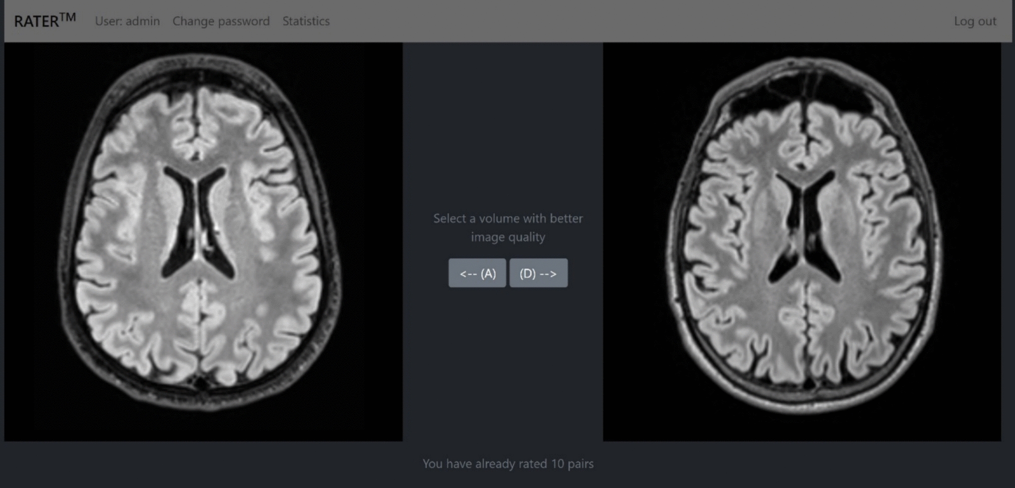
Expert ratings

All the reconstructions were stored in DICOM format for subjective rating of image quality. Two experienced interventional neuroradiologists (J.S., B.E.) with 23 and 17 years of experience and one experienced pediatric neuroradiologist (S.R.) with 14 years of experience were asked to subjectively rate the CIRIM and CS images on multiple categories. The raters were blinded to the diagnosis of the cases whose images were processed for the study. The raters were only asked to review the FLAIR sequence. They scored images side-by-side on multiple categories on a 1 to 5 image quality scale. The scores were as follows: 1 for non-diagnostic quality, 2 for poor quality, 3 for acceptable quality, 4 for good quality, and 5 for excellent quality. The order of the reconstruction methods was randomized, and the raters remained unaware of the method used and the patients’ clinical information. Inspired by previous work, five scoring categories were adopted. Imaging artifacts related to aliasing resulting from image acceleration, ranging from excessive artifacts that severely degrade images to no artifacts present. Perceived spatial resolution referred to image sharpness and the ability to discern small structures down to the voxel level sharpness, ranging from unacceptable, extreme blur levels to a high level of detail at the native level of the defined spatial resolution. Anatomic conspicuity ranged from being unable to discern (small) anatomical and pathological structures to perfect identification of structures. Diagnostic confidence summarized the certainty in the diagnosis of pathology, e.g., a lesion, on a scan, ranging from being unable and highly uncertain in diagnosis to perfect ability to diagnose a scan. Image contrast referred to the relative difference in the intensity of known tissue types and pathology ranging from no contrast visible to extremely good contrast [3, 22]. After the individual rating of the data, a review meeting was held with the readers, in which selected subjects with discrepancies in reading scores were re-evaluated.

Quantitative analyses

Since a fully sampled scan of the patient data is lacking, we calculated self-referenced quantitative measures of image quality using MRI Quality Control (MRIQC) [23]. Specifically, we selected the following set of metrics that we deemed relevant for the task of image reconstruction: coefficient of joint variation (CJV) [24], signal-to-noise ratio, a quality index (QI1) of the proportion of voxels corrupted by artifacts [25], the entropy focus criterion (EFC), being the Shannon entropy of voxel intensities as an indication of ghosting and blurring induced by head motion [26], the foreground to background energy ratio (FBER), being the mean energy of image values within the head relative to outside the head [27], and the full width at half maximum (FWHM) of the spatial distribution of the image intensity values in units of voxels [28]. To assess the dependency of FWHM on SNR, Gaussian noise was added post hoc to one randomly selected CIRIM reconstruction and FWHM was recalculated.

To study the effect of acceleration factors on the reconstruction of patient data containing pathology, we trained a CIRIM on FLAIR scans adopted scans from the FastMRI dataset [29]. The training set consisted of 344 scans and the validation set consisted of 107 scans. The model was trained on a range of acceleration factors from 4 × to 10x. Details on the dataset and training are reported elsewhere [20]. For evaluation, we computed the structural similarity (SSIM) index over the entire validation set for all acceleration factors. Furthermore, we selected a subset of 10 patients for which labeled lesion locations were available [30]. For all acceleration factors, we computed the contrast ratio (CR) as (Ilesion-IWM)/IWM with Ilesion and IWM being the median intensities in bounding boxes in the lesion and in white matter, respectively. We computed repeated-measures ANOVA to test for an effect of the acceleration factor on the SSIM and CR values.

In 10 randomly selected patients with a visible lesion of heterogeneous origin, a region of interest was manually annotated within the lesion and in white matter proximal to the lesion. CR was computed in both the CIRIM and the PICS reconstructions. A Wilcoxon signed-rank difference test was performed.

Statistics

Statistical analyses were performed using SciPy [31]. The statistical significance threshold was set at p < 0.01 for all tests. Bonferroni correction for multiple comparisons was used when necessary. A one-sample Wilcoxon signed-rank test was used to determine whether the expert scores significantly preferred one over the other reconstruction method. A paired t-test was used to determine whether the SNR differed significantly between methods. Probabilistic ordinal linear regression was performed to evaluate the interaction effect of higher image resolution on improved rating scores, depending on the reconstruction method used. The voxel volume was used as image resolution metric. For each reconstruction method and per patient group, post hoc one-sample Wilcoxon signed-rank tests were used to determine significance at a Bonferroni-corrected threshold over multiple scoring categories.