Database

We use the MCYT [15] signature subcorpus, a component of the MCYT baseline corpus, designed to evaluate online handwritten signature recognition and verification systems. Below are its key characteristics:

Acquisition: Signatures are captured using a WACOM Intuos A6 USB tablet, which records \( X \) and \( Y \) coordinates (position), pressure (\( p \)) applied by the pen, as well as its azimuth and altitude angles. Signature is sampled at 100 Hz and 2540 lines per inch.

Participants: The database included participation from 330 individuals.

Authentic Signatures: Each participant provided 25 genuine signatures.

Skilled Forged Signatures: Each participant also submitted 25 forgeries, performed with skill.

To illustrate the process of watermarking in the context of online handwritten signals, we represent the signal and the watermarks as follows:

Let \(\textbf =[X, Y] = \begin x[1] & y[1] \\ x[2] & y[2] \\ \vdots & \vdots \\ x[N] & y[N] \end\) be an \(N \times 2\) matrix representing the online handwritten signal, where x[n] and y[n] are the X and Y spatial coordinates of the n-th point in the signal, respectively.

Two binary watermarks, \(w_x, w_y \in \^N\), are randomly generated. When combined, they form an \(N \times 2\) matrix, where the first column corresponds to \(w_x\) and the second column corresponds to \(w_y\). In a specific application, the bits may represent relevant information, such as an encrypted timestamp or secret code. However, for this experiment, the content of the watermarks is not relevant.

DCT Watermarking

The DCT technique is particularly advantageous due to its ability to compact signal energy into a few coefficients, which facilitates imperceptible watermark embedding. The watermarking process in the discrete cosine transform (DCT) domain is described as follows.

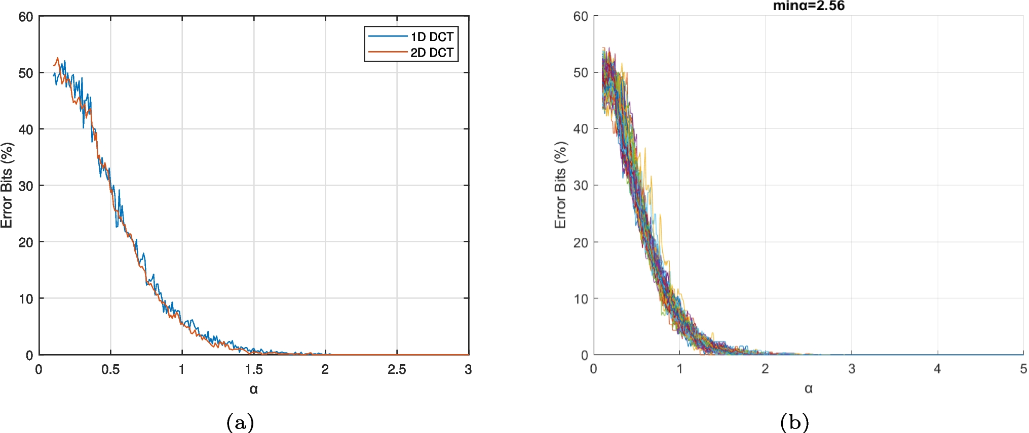
Fig. 1

Relevance of \(\alpha \) in percentage of error bits in the watermark (a). Comparison of 1D and 2D DCT transform for a sample user (b). Overlapped 1D DCT results for all the users

Watermark Insertion

The handwritten signal is transformed into the frequency domain using the two-dimensional discrete cosine transform (DCT2):

$$\begin \textbf_} = \text (\textbf), \end$$

(1)

where \(\textbf_} \in \mathbb ^\) is the matrix of 2D DCT coefficients of the X and Y coordinates of the signal.

Alternatively, for the one-dimensional DCT, we apply the DCT separately to the X and Y coordinates:

$$\begin \textbf_x = \text (X), \quad \textbf_y = \text (Y), \end$$

(2)

These individual 1D DCT results are then concatenated column-wise to form a 2D DCT matrix:

$$\begin \textbf_} = \left[ \textbf_x, \textbf_y\right] \in \mathbb ^. \end$$

(3)

The watermarks are embedded into the DCT coefficients of the original signal as follows:

$$\begin \textbf_} = \textbf_} + \alpha \cdot \textbf, \end$$

(4)

where \( \alpha \) is a scaling factor that controls the watermark strength in the DCT coefficients, and

$$\begin \textbf = \begin w_x&w_y \end \in \mathbb ^, \end$$

(5)

is the watermark matrix, formed by combining the two binary watermarks \(w_x\) and \(w_y\).

After embedding the watermark in the frequency domain, the modified signal is transformed back to the spatial domain using the inverse discrete cosine transform (IDCT):

$$\begin \textbf_} = [X_w, Y_w] = \left\lfloor \text (\textbf_}) + 0.5 \right\rfloor \end$$

(6)

where \( \left\lfloor \cdot \right\rfloor \) represents the floor function, but adding 0.5 before applying it effectively rounds to the nearest integer, ensuring the sample values remain integers.

The result, \(\textbf_}\), is the signal with the watermark embedded, where the X and Y coordinates have been slightly altered to \(X_w\) and \(Y_w\), respectively.

Watermark Extraction

The watermark can be extracted by comparing the DCT coefficients of the original signal and the watermarked signal. The difference between the DCT coefficients is scaled by the factor \(\alpha \) to recover the original watermark:

$$\begin \textbf_} = \frac_} - \textbf_}}. \end$$

(7)

Here, \(\textbf_}\) represents the recovered watermark. It is then rounded to integer values to obtain the final representation of the watermark:

$$\begin \textbf_} = \left\lfloor \textbf_} + 0.5 \right\rfloor . \end$$

(8)

Before applying the DCT watermarking, some adjustments are required to ensure the watermark is properly embedded and extracted.

Fig. 2

Example of x[n] and y[n] coordinates for a signature, along with their watermarked counterparts \(x_w\)[n], \(y_w\)[n], and the corresponding differences(a)for \(\alpha \) =10 (b) for \(\alpha \) = 100

Minimum \(\alpha \) Value Determination for DCT

To determine the minimum \(\alpha \) value required for watermark recovery without errors, a brute-force procedure is employed. For a given sample signature, the \(\alpha \) value is adjusted within the range \([0.1:0.01:3]\). Naturally, results can vary across different users, so this process is repeated for the entire set of users.

Figure 1a illustrates the error percentage for each tested \(\alpha \) value, alongside a comparison between one-dimensional (1D) and bidimensional (2D) transforms. It is evident that there are no errors in the detected watermark for \(\alpha > 2\). Furthermore, the results for 1D and 2D DCT are very similar, which is expected, as the signal is nearly one-dimensional (\(N \times 2\), where \(N \gg 2\)). For simplicity, we opted for the 1D transform.

Figure 1b displays the plots for the 330 users, overlaid to show the minimal variability between them. An \(\alpha \) value of 2.56 is the minimum required to ensure error-free watermark extraction for all users.

Figure 2 shows the x and y coordinates for both the original and watermarked signatures, along with the corresponding differences between their respective values. Unlike our previous results based on difference expansion [8], where distortions were concentrated in the latter part of the signature, where writing speed is higher, the current approach results in more evenly distributed errors across the entire signature. The watermarking process now introduces errors that are more uniformly spread, leading to a more consistent effect across both the x and y axes, and ultimately, reducing localized distortion

DWT Watermarking

The wavelet decomposition of a one-dimensional signal generates bands or components divided into two main groups at each decomposition level:

Approximations (A): These represent the smoothed version of the original signal, containing the low-frequency information (global trends) of the signal.

Details (D): These capture the rapid variations or details of the signal, corresponding to the high-frequency components removed from the approximation.

At each decomposition level, the original signal undergoes the following steps:

1.

The signal is passed through a low-pass filter to generate the approximation component A.

2.

Simultaneously, the signal is passed through a high-pass filter to generate the detail component D.

3.

Both components (A and D) are then downsampled by a factor of 2 to reduce the data size.

This process can be repeated for multiple levels, with each level further decomposing the approximation component obtained from the previous level. The multi-resolution capability of DWT enables selective embedding, making it particularly robust to compression and noise.

The watermarking process in the discrete wavelet transform (DWT) domain is described as follows.

Watermark Insertion

The handwritten signal is decomposed into wavelet coefficients using the Haar wavelet:

$$\begin A_x, D_x = \text (X), \quad A_y, D_y = \text (Y), \end$$

(9)

where \( A_x \) and \( A_y \) are the approximation coefficients, and \( D_x \) and \( D_y \) are the detail coefficients of the X and Y coordinates, respectively. Figure 3a illustrates an example of an original signature and its approximation and detail decompositions.

Two binary watermarks, \( w_x, w_y \in \^ \), are randomly generated, corresponding to the size of the wavelet coefficients.

Fig. 3

a Approximation and detail bands of the wavelet decomposition. b Minimum \(\alpha \) value for recovering error-free watermark

These watermarks are embedded into the approximation coefficients as follows:

$$\begin A_ = A_x + \alpha \cdot w_x, \quad A_ = A_y + \alpha \cdot w_y, \end$$

(10)

where \(\alpha \) is a scaling factor controlling the watermark strength.

After embedding, the watermarked signal is reconstructed using the inverse DWT:

$$\begin s_ \!=\! \left\lfloor \text (A_, D_x) + 0.5 \right\rfloor , \quad s_ = \left\lfloor \text (A_, D_y) + 0.5 \right\rfloor . \end$$

(11)

The result, \(\textbf_} = \begin s_&s_ \end\), is the signal with the watermark embedded.

Watermark Extraction

The watermark can be extracted by decomposing the watermarked signal into wavelet coefficients:

$$\begin A_, D_ \!=\! \text (s_), \quad A_, D_ = \text (s_). \end$$

(12)

The embedded watermarks \(w_x\) and \(w_y\) are then recovered by comparing the wavelet coefficients of the original and watermarked signals:

$$\begin \hat_x = \frac - A_x}, \quad \hat_y = \frac - A_y}. \end$$

(13)

Finally, the extracted watermarks \(\hat_x\) and \(\hat_y\) are rounded to integer values to obtain their binary representation:

$$\begin \hat_x = \left\lfloor \hat_x + 0.5 \right\rfloor , \quad \hat_y = \left\lfloor \hat_y + 0.5 \right\rfloor . \end$$

(14)

Minimum \(\alpha \) Value Determination for DWT

We applied the same procedure described in the “Minimum \(\alpha \) Value Determination for DWT” section. Figure 3b shows the obtained result. The minimum \(\alpha \) value that ensures zero errors for all users is \(\alpha = 0.71\). The rapid drop in error when \( \alpha \) is around 0.7 is due to the threshold at which the watermark strength becomes sufficient for reliable extraction. Below this threshold, the watermark is too weak to be distinguished from noise, leading to a high error rate. Once \( \alpha \) surpasses this critical point, the watermark signal is strong enough to be extracted accurately, resulting in a sharp decline in errors. Additionally, quantization can also affect the shape of the watermark, as it introduces rounding errors that may alter the exact values, further influencing the extraction accuracy.

Distortion Calculation

To evaluate the impact of the watermark on the original signal, two common metrics are used: mean squared error (MSE) and mean absolute error (MAE):

$$\begin \text _} = \frac \sum _^ \left( \textbf_i - \textbf_,i} \right) ^2, \end$$

(15)

$$\begin \text _} = \frac \sum _^ \left| \textbf_i - \textbf_,i} \right| , \end$$

(16)

where \(\textbf_i\) and \(\textbf_,i}\) are the X and Y coordinate values of the original and watermarked signals at the i-th point.

Fig. 4

a MAE for different \(\alpha \) values and inserted bits n. b Minimum \(\alpha \) value determination for different inserted bits n

Multi-bit DCT Watermarking

While prior DCT watermarking techniques primarily focused on single-bit embedding per sample, our approach extends this by encoding multiple bits per sample, effectively increasing payload capacity while maintaining an acceptable trade-off between robustness and imperceptibility. The key modification is in the watermark embedding process, where n-bit watermark values are mapped onto DCT coefficients, rather than using a binary insertion scheme. This leads to a controlled and predictable increase in distortion, as analyzed in the “Derivation of the SNR Impact due to n and \(\alpha \)” section. We define the following additional variables:

\(\textbf = [w_x, w_y]\): Watermark vectors for x and y, where each element of \(w_x\) and \(w_y\) is a random integer in the range \([0, 2^n - 1]\).

n: The number of bits used to encode each sample in the watermark.

\(\text \): The fraction of incorrect bits in the extracted watermark relative to the original watermark.

Watermark Embedding Process

The watermark embedding process follows the same steps as for single-bit DCT watermarking, with the key difference being that, in this case, multiple bits per sample are encoded into the DCT coefficients, allowing for a higher payload capacity. Specifically, the watermark values are represented as integers.

Table 2 Minimum MAE for \(\alpha =2.56\) for different values of n

The process is as follows:

1.

Apply discrete cosine transform (DCT) to the \(X\) and \(Y\) coordinates (2) and (3).

2.

Embed the watermark into the DCT coefficients (4).

3.

Apply inverse DCT (IDCT) to recover the watermarked signal (6).

Watermark Extraction Process

The watermark extraction process follows a similar approach, where the watermark is recovered by comparing the DCT coefficients of the watermarked and original signals. Specifically, the difference between the DCT coefficients is scaled by the factor \(\alpha \) to retrieve the original watermark:

$$\begin \hat}_} = \frac(X_w) - \textbf(X)}, \quad \hat}_} = \frac(Y_w) - \textbf(Y)}. \end$$

(17)

Here, \(\hat}_}\) and \(\hat}_}\) represent the recovered watermark components. These values are then rounded to integer values to obtain the final binary representation of the watermark:

$$\begin \hat}_} \!=\! \min \left( \left\lfloor \hat}_}+0.5 \right\rfloor , 2^n - 1\right) , \quad \hat}_} = \min \left( \left\lfloor \hat}_}+0.5 \right\rfloor , 2^n - 1\right) . \end$$

(18)

Multi-bit Metrics Calculation

To evaluate the performance of the watermarking process, we use the following metrics:

1.

Mean absolute error (MAE): Refer to (16). Figure 4a shows the MAE for different numbers of inserted bits (n) and \(\alpha \) values. A linear increase is observed, with a steeper slope as n increases. This rapid growth for large n values limits the maximum number of bits per sample to n = 5. Table 2 presents the MAE values obtained for \(\alpha =2.56\) across several n values. It can be observed that the MAE approximately doubles with the addition of each new bit.

2.

Percentage error in watermark extraction: To calculate the percentage error in watermark extraction, follow these steps:

1.

Convert the original and extracted watermarks to binary representations:

$$\begin w_x^}, \quad \hat_x^}, \quad w_y^}, \quad \hat_y^}. \end$$

(19)

2.

Perform the exclusive OR (XOR) operation to count the differing bits:

$$\begin \text _x = \frac w_x^} \text \hat_x^}}, \quad \end$$

(20)

An analogous equation is applied for the \(y\)-coordinates.

3.

Compute the average percentage error:

$$\begin \text = \frac_x + \text _y} \cdot 100. \end$$

(21)

Figure 4b shows the percentage of error bits for different numbers of inserted bits (n) and \(\alpha \) values. We observe that the minimum \(\alpha \) value for zero-error watermark recovery is not significantly affected by the number of inserted bits n.

Derivation of the SNR Impact due to n and \(\alpha \)

Now, we will derive the impact of the watermark on the signal-to-noise ratio (SNR), considering the definitions and variables introduced earlier.

Noise Power due to the Watermark

The watermark values are uniformly distributed between 0 and \(2^n - 1\). The variance of a uniform random variable \(X \sim U(0, 2^n - 1)\) is given by the following:

$$\begin \text (X) = \frac. \end$$

(22)

Since the watermark is embedded in both the X and Y coordinates, the total watermark power for both dimensions is as follows:

$$\begin P_} = \frac. \end$$

(23)

The watermark-induced noise power is scaled by the embedding strength \(\alpha \):

$$\begin P_} = \alpha ^2 \cdot \frac. \end$$

(24)

Impact of Watermark on SNR

The impact of the watermark on the SNR is the relative change in SNR due to the added noise. Assuming the original SNR is dominated by \(P_}\), the SNR degradation (impact) is given by the following:

$$\begin \text = -10 \cdot \log _(P_}). \end$$

(25)

The impact of the watermark on SNR can be broken down as follows:

1.

The impact of \(\alpha \) is quadratic, as shown by the \(-20 \cdot \log _(\alpha )\) term.

2.

The impact of n is also quadratic, as the watermark power grows with \((2^n - 1)^2\), leading to the \(-20 \cdot \log _(2^n - 1)\) term.

3.

The constant term \(+10 \cdot \log _(6)\) comes from the scaling factor of the watermark power.

This complete analysis of the watermark impact on SNR considers both the number of bits n and the embedding strength \(\alpha \).

Fig. 5

a \(\alpha \) effect on SNR b effect of additive noise on \(\alpha \)

Figure 5a illustrates the impact of \(\alpha \) and the number of inserted bits n on the SNR of the watermarked signal. We observe a strong deterioration of SNR for large n values and embedding strengths (\(\alpha \)).

Tolerance to Noise

Figure 5b illustrates the impact of additive continuous uniform noise on the percentage of error bits in the decoded watermark. We observe that DCT watermarking demonstrates a notable tolerance to noise without significantly affecting watermark decoding. However, this robustness necessitates a stronger watermark embedding, achieved by increasing the alpha value.

Feature Extraction

The signature components, including the \( x \) and \( y \) coordinates and \( p \) pressure values, are normalized so that their mean is zero and their standard deviation is one. After normalization, the first and second derivatives of the signature are computed to extract dynamic features. The process for feature extraction involves the following steps:

First derivative (velocity): The first derivative is calculated using a window length of 11 points [16]. It represents the velocity of the signature in the \( x \), \( y \), and pressure directions:

$$\begin \dot = \frac, \quad \dot = \frac, \quad \dot = \frac \end$$

(26)

Second derivative (acceleration): The second derivative is computed to capture the acceleration:

$$\begin \ddot = \frac, \quad \ddot = \frac, \quad \ddot = \frac \end$$

(27)

The first and second derivatives are normalized by subtracting their respective means and dividing by their standard deviations and then concatenated to form the final feature vector \( \textbf_n \):

$$\begin \textbf_n = \left[ x_n, y_n, p_n, \dot_n, \dot_n, \dot_n, \ddot_n, \ddot_n, \ddot_n \right] \end$$

(28)

This vector is computed for each signal sample.

Recognition Algorithm

The recognition process begins by modeling each user using five genuine signatures as the training set. For each testing signature, the Dynamic Time Warping (DTW) [17] distance is computed between the testing signature and each of the five training signatures. The final distance is obtained as the minimum value from the five computed distances.

Fig. 6

Impact of \(\alpha \) in recognition accuracies (a). Identification (b) min DCF verification error

There are two possible recognition modes [18]:

Identification: The DTW distance computation is repeated for the N user models, and the model that provides the minimum distance corresponds to the recognized user.

Verification: Only one DTW distance is obtained, comparing the testing signature with the claimed identity model. If the distance is below a decision threshold, the user is positively verified. Otherwise, the user is considered an impostor. Threshold setup and the experimental determination of verification accuracy, measured by the minimum detection cost function (minDCF), are based on [19].