The sample comprised a total of 190 healthy individuals, 93 males and 97 females, recruited from FIDMAG Hermanas Hospitalarias Research Foundation through public advertising in the province of Barcelona. All participants met the following inclusion criteria: not having a current or antecedent history or first-degree family history of psychiatric disorders; European ancestry; age between 18 and 65 years old; right-handedness; and estimated intelligence quotient (IQ) > 70, assessed with the Test de Acentuación de Palabras (TAP) [40], an adapted Spanish version of the National Adult Reading Test (NART) [41]. Exclusion criteria included drug or alcohol abuse and a history of neurological damage. All participants provided written consent after being informed about the study procedures and implications.

The sample characteristics are provided in Table 1. No significant differences between males and females regarding age (Student’s t-test, t = -1.265; p = 0.2) and TAP (Student’s t-test, t = 0.02; p = 0.99) were found.

All participants underwent a neuroimaging protocol in a 1.5 Tesla GE Sigma scanner at Hospital Sant Joan de Déu (Esplugues de Llobregat, Spain). High-resolution T1 weighted (T1w) head magnetic-resonance images (MRI) were obtained with the following acquisition parameters: matrix size 512 × 512; 180 contiguous axial slices; voxel resolution 0.47 × 0.47 × 1 mm3; echo (TE), repetition (TR) and inversion (TI) times, (TE/TR/TI) = 3.93ms/2000ms/710ms, respectively; and flip angle 15º.

T1w MRIs were processed through the recon-all pipeline of FreeSurfer (v. 5.3), which included motion correction, removal of non-brain tissue, automated Talairach transformation, tessellation of the grey and white matter boundaries and topological correction to rectify holes, intersections and isolated vertices. The triangulated mesh representing the cortical surface was achieved using a deformation algorithm, and the mean surface area and mean cortical thickness were obtained for all subjects. All the images included in this study complied with the standardized quality control protocols from the ENIGMA consortium (http://enigma.ini.usc.edu/protocols/imaging-protocols).

The sulcal pits were extracted from the mesh of the white matter surface for each hemisphere, using the process “Sulcal pits extraction” implemented in BrainVisa 4.5 (https://brainvisa.info/web/). The process is detailed in Auzias et al. [31].

Briefly, a depth map was first generated by using the Depth Potential Function (DPF) [42]. Then, a watershed algorithm divided large sulci into sulcal basins based on ridge height (R), basin area (A), and the geodesic distance between two pits (D). The parameters of group Fiedler length (gFL) and group average surface area (gSA) were calculated based on our sample values to optimize the process, as suggested in Auzias et al. [31], obtaining averaged values between hemispheres of gFL = 219.84 mm and gSA = 81625.11 mm2. On the other hand, the default thresholds of ridge height (ThrR), area (ThrA) and distance (ThrD) for basin merging implemented in BrainVisa (ThR = 1.5 mm, ThD = 20 mm, ThA = 50 mm2) were maintained due to their proven good performance for sulcal pits extraction [31]. The use of DPF for the extraction of sulcal pits ensures that the procedure is independent of brain size, as it does not affect the computation of depth in this method [31]. Furthermore, to ensure that noisy pits were not extracted on the bumps of shallower sulci, a restriction to consider exclusively sulcal pits with positive DPF values was applied.

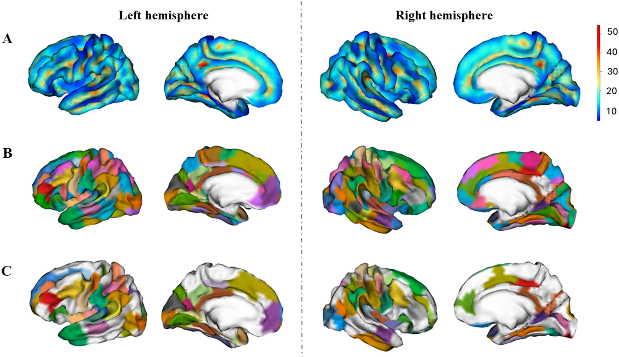
To compare the differences in sulcal pits between sexes, we applied the method depicted in [31]. An areal map, consisting in the parcellation of the brain in smaller regions, was built considering all individuals, both males and females, so that each group equally contributed to the final parcellation. First, the sulcal pits maps were smoothed using a full-width half-maximum (FWHM) of 5 mm, maintaining the peak value at one, by using the BrainVisa process “Pits Texture Smoothing”. Second, the smoothed pits’ maps of both hemispheres were projected to the corresponding hemisphere of the Freesurfer fsaverage4 template. Third, all the individual sulcal pits maps were summed to obtain a group density map, showing the probability of sulcal pits at each vertex (Fig. 1A). Fourth, the BrainVisa process “Group Watershed” with the default parameters (ThR = 2 mm, ThD = 15 mm and ThA = 100 mm2) was applied to the density map to obtain the group areals (Fig. 1B). In all, 98 areals were mapped in the left hemisphere and 101 in the right.

Finally, the individual sulcal pits maps were projected into the parcellated template. As expected, due to methodological constraints, although most individuals presented one sulcal pit in each areal, some did not present any or more than one [31]. Therefore, only those areals with at least a frequency of one sulcal pit in 80% of the sample were retained for further analysis (49 for the left hemisphere and 47 for the right) (Fig. 1C). As established in previous studies, this criterion ensures that the analyses of the differences in sulcal pits are performed in the most reproducible sulci across individuals, the primary sulci, which are the first sulci to emerge [21, 32, 43].

Subsequently, to provide biological meaning to the sulcal pits on those areals, we used the Destrieux atlas [44] to describe the anatomy of the cortical regions comprised by each areal. In addition, the Brodmann atlas, as implemented in MRIcro [45], was used to determine the Brodmann area (BA) correspondence of the areals. In Supplementary Materials 1, Tables S1 – S2, a detailed description of the fsaverage4 coordinates (MNI305) comprised in each areal and their correspondence to Destrieux atlas and BA is provided for the left and right hemispheres.

Density and areals maps. After individual extraction of sulcal pits, the individual maps were smoothed and summed to obtain a density map, showing the probability of sulcal pits occurrence in the whole sample (A). Then, a watershed algorithm was applied to obtain the map of the areals (B). Finally, those areals in which at least 80% of the sample presented at least one sulcal pit were selected for further analyses (C)

To perform a refined analysis of the differences in sulcal pits related to the different stages of prenatal brain development, we classified areals into three groups based on their depth, applying a k-means algorithm as presented in Li et al. [36]. With this methodology the areals are aligned accordingly with the temporal emergence of the sulci within them. In accordance with previous studies, the deepest areals are presumed to contain the earliest-emerging sulci, while the shallowest comprise the later-emerging ones [24, 36].

K-means was performed considering the maximum depth values of the sulcal pits of all individuals in each areal, and not the average DPF value of the areal as in Li et al. [36], ensuring that the captured depth value corresponded to the fundi of the cortex and was not distorted by values of other vertices present on gyri. If an individual did not present a sulcal pit in a determined areal (7.18% of cases in the left hemisphere and 7.67% in the right hemisphere), this value was filled with the group-average DPF of the sulcal pits in that areal. When an individual presented more than one, the value of the deepest pit was considered (27.19% of cases in the left hemisphere and 26.91% in the right hemisphere). K-means was conducted with three classes (k = 3) and 100 iterations were performed. As a result, we obtained the classification of each areal in one of the 3 depth clusters (deep, intermediate and shallow) for each hemisphere. The results of the k-means are provided in Supplementary Materials 2, Figure S1 and Table S1 correspond to the left hemisphere and Figures S2 – S3 and Tables S2 – S3 to the right hemisphere. Greater values of DPF represent greater depths. Therefore, areals classified in the deepest cluster would exhibit higher DPF values compared to those classified in the intermediate and shallow clusters. For clarity, henceforth, DPF will be referred to as depth.

For the left hemisphere, the deep cluster comprised 20 areals, the intermediate 18 and the shallow 11. In the case of the right hemisphere, the deep cluster comprised 17 areals, the intermediate 20 and the shallow 9. In Fig. 2, a visualization of the areals comprised in each cluster is presented.

Supplementary Materials 1 provides a table of the classification of the areals and their mean depth for the left and right hemispheres (Table S5 and Table S6, respectively).

Representation of the areals in each depth cluster for the left and right hemispheres. Areals classified in the deep cluster are represented in orange, those in the intermediate cluster in blue and the shallowest areals are in pink. The medial and outer parts of the cortex are displayed (left and right parts of the figure, respectively). Non-colored regions contain areals where fewer than 80% of individuals had a sulcal pit

To address our first objective, we examined sex differences in the frequency of sulcal pits at the hemispheric level.

First, we conducted linear regression analyses with the total number of sulcal pits per hemisphere as the dependent variable. In a first model, we included sex as the main factor, and, as covariates, age, estimated IQ, and estimated intracranial volume (ICV, defined as the total volume in the cranial cavity). Despite the stability of sulcal pits across the lifespan, we included age as a covariate due to its influence on overall variability in brain anatomy [46,47,48] and the potential indirect effects it may have on sulcal pits measurement. The inclusion of the estimated IQ was based on previous findings suggesting its influence on sulcal pits frequency [49]. Although pit depth may be relatively unaffected by brain size [31], sulcal pits frequency could vary with ICV. Moreover, considering the well-established sex differences in brain size [50], adjusting for ICV was essential. In a second model, we extended the analysis to explore the interaction between sex and age (sex x age), while retaining the same covariates. This allowed us to assess whether the relationship between sex and sulcal pits frequency varied across age at brain scanning.

Second, we analyzed the correlation between sulcal pits and additional neuroanatomical cortical metrics at the hemispheric level by first adjusting the mean surface area and mean cortical thickness values for ICV to mitigate potential distortions in the analyses stemming from differences in brain size between groups. To do so, a linear regression model was employed, considering mean surface area or mean cortical thickness as the dependent variables and ICV as the independent variable. The residuals of that model were then retained for subsequent analyses. Next, we used a regression model to test the correlation between the number of sulcal pits at the hemispheric level and the surface area within the corresponding hemisphere. This analysis was performed in the sex-pooled sample and stratifying the sample by sex. The same procedure was applied in the case of mean cortical thickness. Age and estimated IQ were considered as covariates and a second model to explore the interaction between age and sex was also built.

A post-hoc power analysis indicated that, with our sample size, we had 80% power to detect significant effects of sex on the number of sulcal pits for a ß of at least ± 1.629.

Regarding our second objective, we explored the potential temporal window during which differences in the frequency of sulcal pits may have emerged. Therefore, we calculated the total number of pits in the areals conforming the depth, intermediate and shallow clusters. Then, a linear model was built considering the total number of pits in each depth cluster as a dependent variable, sex as the main factor and age, estimated IQ, and ICV as covariates. A second linear model, including the interaction between age and sex, was also performed.

Subsequently, we analyzed sex differences in sulcal pits depth for each areal to topographically identify the anatomical and functional regions where these differences may be localized. First, the interquartile range (IQR) method was applied to detect potential outlier depth values in each areal and those individuals whose depth values were above or below 1.5*IQR (~ 2.7 standard deviations) were excluded. In Supplementary Materials 1, Tables S15 – S16, the percentage of outliers in each areal is presented. Next, a linear model was built considering sulcal pit depth in each areal as the dependent variable, sex as the main factor and age and estimated IQ as covariates.

For all models, we report both the raw p-value (p) and the multiple comparisons adjusted p-value (pFDR) obtained with the False Discovery Rate (FDR) method [51]. Statistical significance was established at pFDR < 0.05. The statistical analyses were performed using R (v. 4.3.2) [52] and the results on the brain templates were plotted using fsbrain R package [53].