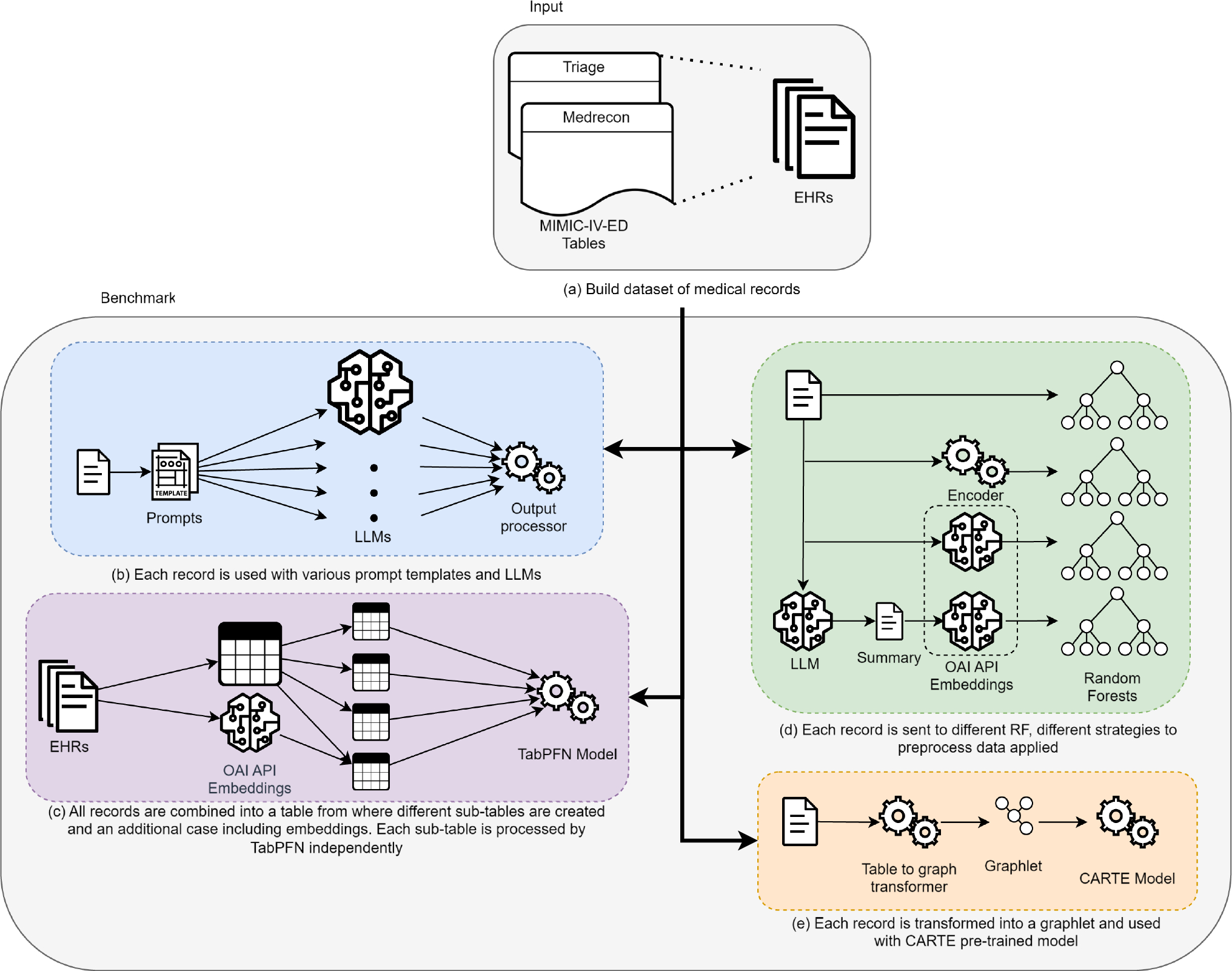
Overview denoting successive process steps. RGB and depth data are acquired (B) using an Intel RealSense camera. Live segmentation (C) of the target organ, based on the SAM-Track approach, is initialized by the manual choice of six seed points in AR (A2). A sensor point cloud (target) is cropped from the total point cloud using the resulting segmentation mask, and a model point cloud is derived from the organ’s CT scan (source). Following an initial pre-alignment (A1) performed by the user, the source point cloud is registered onto the target point cloud (D) in all consecutive frames. Based on the resulting transformation, algorithmic latency is bypassed by forecasting (E, orange) one frame ahead. A virtual 3D model of the CT volume is projected (F) at the registered position using Microsoft HoloLens 2

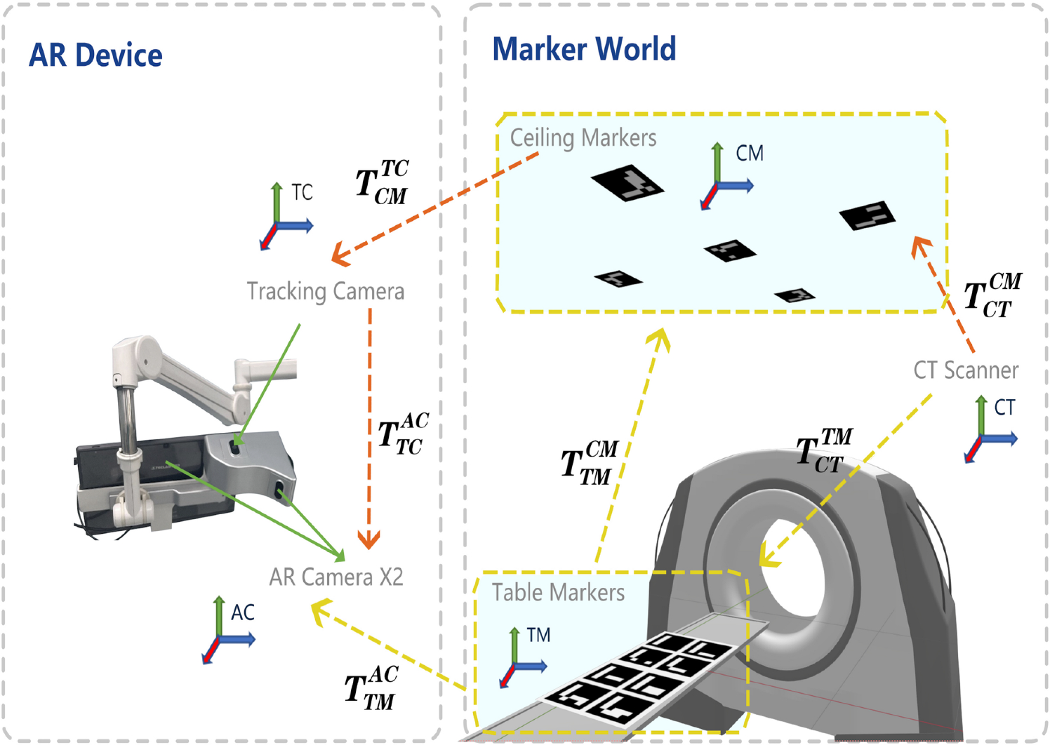
As indicated in Fig. 1, our approach decouples the visualization from the registration, as AR HMDs currently have limitations in terms of precise depth sensing. Hence, we utilize the HoloLens 2 HMD (Microsoft) for visualization and interaction, while employing the RealSense D415 RGB-D camera (Intel) as a high-definition 3D-sensing device. Figure 2 consolidates our process to establish a foundation model based and low-latency AR navigation method applied to open liver surgery. The individual phases and steps are described in the following subsections.

To enable robust segmentation and registration even in challenging clinical situations, we propose an approach with minimal user interaction comprising two steps, which require approximately 20 s in total.

(1) At present, automatic global registration of the liver organ is still challenging due to the lack of distinct features, especially under high levels of occlusion [5, 6]. However, this registration is crucial for later clinical practice and creates a significant demand for quality control. Hence, the surgeon is instructed to roughly pre-position a virtual model of the liver’s CT scan to its real-world counterpart (Fig. 2, step A1), ensuring a maximum distance of approximately 10 cm between the visible margins. We provide the intuitive HoloLens 2 hand interface to enable a rapid pre-alignment between both structures. The subsequent initial transform (\(T_^(0)\)) of the virtual liver model (L) substitutes for a global registration from the perspective of the HoloLens (H), while incorporating the surgeon’s expertise regarding the organ’s structure.

(2) Establishing robust segmentation of organs is challenging, especially in complex clinical scenarios involving a liver with an irregular or split structure. To better guide the unchanged SAM foundation model in assisting with this task, prior information in the form of prompts is required. Hence, we instruct the surgeon to place six seed points \(s_\) directly in AR, each three ones onto the target organ (’positive’), and onto its surroundings (’negative’) (Fig. 2, step A2). Similar to [12], we developed a HoloLens 2 application enabling the user to select arbitrary seed points using finger tracking.

We acquire high-resolution RGB and depth streams from the Intel RealSense and stream these data to a workstation (Fig. 2, step B). In the initial frame, the offset transform \(T_^\) between the HoloLens (H) and the RealSense (R) is calibrated using an ArUco chart [13] (C) placed in the field of view of both sensors. Hence, \(T_^\) is calculated as \((T_^)^ \cdot T_^\). The ArUco chart can be removed after recording the first frame due to the inside-out tracking capabilities of the HoloLens.

To detect the liver in each RGB frame, we employ the SAM-Track approach (unpublished work by Cheng et al.) (Fig. 2, step C), which builds upon SAM [9] by incorporating the Decoupling Features in Hierarchical Propagation (DeAOT) tracker [14] to achieve high frame rates. We utilize the RGB image coordinates of the three ’positive’ and the three ’negative’ seed points \(s_\), placed in step A2, as SAM prompts. Each consecutive RGB frame receives a segmentation mask by tracking the initial SAM segmentation using the DeAOT tracker. For performance purposes, our method comprises SAM with a ViT-B backbone and DeAOT with a DeAOTT backbone. Using the depth map from the RealSense camera, a target point cloud is cropped from the total point cloud based on the obtained segmentation mask.

The source point cloud from the liver’s CT model is constructed by sampling 5,000 points and aligned with the target point cloud through rigid point cloud registration (Fig. 2, step D). Similar to [6], we employed a voxel resolution of 5 mm for point clouds, balancing structural and temporal resolution. The registration is initialized with the manual pre-positioning (Fig. 2, step A1), described by \(T_^(0) = T_^(0) \cdot (T_^)^\). In all consecutive frames, the PointToPoint ICP algorithm [15] iteratively updates \(T_^(t)\) using a distance threshold of 1 cm.

We visualize the registration results on the HoloLens (Fig. 2, step F) by transmitting the registration transformation matrix \(T_^(t)\) to the HoloLens app via wireless local network. The app displays a semi-transparent version of the CT model used for registration, which is transformed by \(T_^(t) = T_^(t) \cdot T_^\).

Our proposed data processing pipeline operates with a total latency of approximately 100 ms on the available hardware. As in situ navigation is time critical, the related latency must be as low as possible. Due to its importance in time-series analysis and prior conceptual work demonstrating promising results [16], we investigate Double Exponential Smoothing (DES) [17] (chapter 6.4.3.3) to forecast the next frame’s transformation (Fig. 2, step E). The process result is thereby pre-computed for the consecutive frame, and algorithmic latency is bypassed as a consequence. We translate DES to registration transforms as follows:

$$\begin & \begin S_} =&\,\alpha _ \cdot \vec _ + (1 - \alpha _ ) \cdot (S_} + b_} ) \\ \end \end$$

(1)

$$\begin & \begin b_} =&\,\gamma _ \cdot (S_} - S_} ) + (1 - \gamma _ ) \cdot b_} \\ \end \end$$

(2)

$$\begin & \begin S_} =&\,\alpha _ \cdot \Theta _ + (1 - \alpha _ ) \cdot (S_} \cdot b_} ) \\ \end \end$$

(3)

$$\begin & \begin b_} =&\,\gamma _ \cdot (S_}^} \cdot S_} ) + (1 - \gamma _ ) \cdot b_} \\ \end \end$$

(4)

Forecasting is applied to the translation vector \(\vec _\) and the rotation quaternion \(\Theta _\), both decomposed from a registration transformation matrix T at time t. For each time step, the smoothed value \(S_\) and a trend estimate \(b_\) are calculated. We compute \(\vec _ = S_ + m \cdot b_\) using values calculated by Equation (1) and (2), applying linear interpolation. Similarly, we compute \(\Theta _ = S_ \cdot }^\) using values obtained from Equation (3) and (4), applying spherical linear interpolation to rotation quaternions. For \(m = 1\) time step, we predict the next frame after the frame acquisition gap interval. Forecasting begins with the second frame, where initial values are set as \(S_ = \vec _\) and \(b_ = \vec _ - \vec _\), as well as \(S_ = \Theta _\) and \(b_ = \Theta _^ \cdot \Theta _\).

The data smoothing factor \(\alpha \) and trend smoothing factor \(\gamma \) are optimized via a design-of-experiments study that minimizes the deviation between the forecasted and ground-truth transformation matrices. This deviation is quantified in terms of a Translation Error (TE in Euclidean Distance) and a Rotation Error (RE in Angular Distance). We determine TE and RE for each combination of \(\alpha \) and \(\gamma \) (ranging from 0.0 to 1.0 in increments of 0.1) across three motion scenarios involving a mechanical turning wheel with rotation velocities of 30/15/10 s per turn, respectively. By the high rotation speeds, we simulate rapid organ or sensor movements that may occur during surgical interventions. The liver phantom is positioned on the turning wheel, with its coordinate system off-center, such that the phantom undergoes both rotations and translations. As a reference, we attach an NDI Aurora 5DoF catheter that is tracked using the NDI Aurora system to measure a ground-truth transformation, sampled in accordance with the total latency of our navigation method (100 ms). To optimize the observations to the given problem, we perform regression analysis to estimate the two underlying model functions describing TE and RE dependent on the influencing factors \(\alpha \) and \(\gamma \). We follow the response surface method outlined in [17] (chapter 5.3.3.6—quadratic model, cubic terms neglected). Minimizing these model functions yields the optimum values for \(\alpha \) and \(\gamma \) w.r.t. the real-world reference, as provided in Table 1. These optimized hyperparameters are then substituted into Equation (1)–Equation (4).