Now we use the parametrix constructed in the previous section to establish the necessary \(L^1\) estimates. We first collect some classical results on the well-posedness of second-order parabolic equations with unbounded coefficients.

Proposition 4.1

Consider the Cauchy problem (3.5) satisfying assumptions (3.1)-(3.3). If \(u_0 \in C^\infty (\mathbb ^n)\) satisfies

$$\begin |u_0(x)| \le B e^ \end$$

(4.1)

for some \(B, \beta > 0\). Then for each \(\varepsilon > 0\), there exists \(T_\varepsilon > 0\) and a unique classical solution to (3.5) for \(0 \le t \le T_\varepsilon \) that satisfies

$$\begin |u(x, t)| \le B_\varepsilon e^ \end$$

(4.2)

for some \(B_\varepsilon , \beta _\varepsilon > 0\). Furthermore, u(x, t) is given by

$$\begin e^u_0(x, t):= \int _^n} K(x, y, t; \varepsilon ) u_0(y)\, \textrmy \end$$

(4.3)

for some \(K(\bullet , \bullet , \bullet ; \varepsilon ) \in \mathcal C^\infty (\mathbb ^n_x \times \mathbb ^n_y \times \mathbb _t)\) such that

$$\begin K(x, y, t; \varepsilon ) \le C_\varepsilon \exp \left( -c_\varepsilon \frac \right) , \quad 0 < t \le T_\varepsilon \end$$

(4.4)

for some \(C_\varepsilon , c_\varepsilon > 0\) and \(e^\) satisfies the semigroup property.

The fundamental solution in the case of unbounded coefficients was first constructed in [15]. We refer the reader to [5, §2.2] and [6, §2.4] for proofs of the above proposition and a complete introduction to well-posedness theory for the parabolic Cauchy problem with unbounded coefficients.

We also remark that the dependence on \(\varepsilon \) for the time of existence does not matter for our setting due to the semigroup property; having sufficiently good estimates on the solution at later times will allow us to extend the time of existence.

4.1 Short-Time Estimate

Now we make use of the crucial assumption (3.4) that v(x) is divergence free. This gives us the conservation of mass for the evolution equation (3.5).

Lemma 4.2

Suppose \(u(x, t) \in C^\infty (\mathbb ^n_x \times \mathbb _t)\) satisfies (3.5) and

$$\begin |u(x, t)| \le B e^ \end$$

for some \(B, \beta > 0\). Then,

$$\begin \Vert u(t)\Vert _ \le \Vert u_0\Vert _. \end$$

(4.5)

Proof

By Proposition (4.1), we know that \(u(\bullet , t) \in L^1\). The Fokker–Planck equation preserves positivity [6, §4.1 Theorem 9]. Since v(x) is divergence free, the \(L^1\)-boundedness of the Fokker–Planck evolution follows by decomposing u into positive and negative parts by \(u_0 = u_+ - u_-\), and seeing that

$$\begin \Vert e^u_0\Vert _ \le \Vert e^ u_+\Vert _ + \Vert e^ u_-\Vert _ = \Vert u_+ + u_-\Vert _ = \Vert u_0\Vert _ \end$$

as desired. \(\square \)

Lemma 4.3

Let K(x, y, t) be the fundamental solution from Proposition 4.1. Then,

$$\begin \Vert \partial _y K(\bullet , y, t)\Vert _ \le C(\varepsilon ^2t)^}, \end$$

(4.6)

where C is independent of \(0 < \varepsilon , t \le 1\).

Proof

Using Duhamel’s formula, we see that

$$\begin \partial _y K(x, y, t) = \partial _y K_1(x, y, t) + \int _0^ e^ \partial _y R_2(x, y, s)\, \textrms \end$$

(4.7)

From Lemma 3.4, we see that

$$\begin \Vert \partial _y K_1(\bullet , y, t)\Vert _ \le C(\varepsilon ^2 t)^} \end$$

(4.8)

and

$$\begin \Vert \partial _y R_2(\bullet , y, t)\Vert _ \le C(\varepsilon ^2 t)^}. \end$$

(4.9)

Therefore,

$$\begin \Vert \partial _y K(\bullet , y, t)\Vert _ \le C(\varepsilon ^2 t)^} + \int _0^t (\varepsilon ^2 s)^}\, \textrms \le C(\varepsilon ^2 t)^} \end$$

(4.10)

as desired. \(\square \)

Let \(W^(\mathbb ^n)\) denote the \(L^1\)-based order r Sobolev space. We now show that derivatives of a solution to (3.5) up to a \(\mathcal O(1)\) amount of time independent of \(\varepsilon \) are controlled by derivatives of the initial data.

Proposition 4.4

Suppose \(u(x, t) \in C^\infty (\mathbb ^n_x \times \mathbb _t)\) satisfies (3.5) and

$$\begin |u(x, t)| \le B e^ \end$$

for some \(B, \beta > 0\). Then for every \(r \in \mathbb \), there exists \(0 < \tau _r\le 1\) independent of \(0 < \varepsilon \le 1\) such that for all \(0 \le t \le \tau _r\), u satisfies the estimate

$$\begin \Vert u(t)\Vert _} \le C_\alpha \Vert u_0\Vert _}. \end$$

(4.11)

Proof

For \(r = 0\), Lemma 4.2 gives the desired \(L^1\) estimate. We handle higher derivatives inductively. Assume that the lemma holds for all \(\tilde < r\). Differentiating (3.5), we see that

$$\begin (\partial _t - Q)(\partial _x^\alpha u) = h \nabla \cdot [\partial _x^\alpha , A(x)] \nabla u + [\partial _x^\alpha , v(x) \cdot \nabla ]u, \qquad |\alpha | = r. \end$$

(4.12)

Using Duhamel’s formula, we can write

$$\begin \partial _x^\alpha u = e^(\partial _x^\alpha u_0) + \int _0^t e^ (h \nabla \cdot [\partial _x^\alpha , A(x)] \nabla u(s) + [\partial _x^\alpha , v(x) \cdot \nabla ] u(s))\, \textrms\nonumber \\ \end$$

(4.13)

By assumption v(x), it satisfies 3.3, which means that \([\partial _x^\alpha , v(x) \cdot \nabla ]\) is an order r differential operator with uniformly bounded coefficients. Therefore, by Lemma 4.2, we have

$$\begin \left\| \int _0^t e^ [\partial _x^\alpha , v(x) \cdot \nabla ] u(s)\, \textrms \right\| _ \le C t \max _ \Vert u(s)\Vert _}. \end$$

(4.14)

The remaining term in the integrand of (4.12) is handled using Lemma 4.3. Integrating by parts, we see that

$$\begin&\int _0^t e^ (\nabla \cdot [\partial _x^\alpha , A(x)] \nabla u(s))\, \textrms \\&\quad = \int _0^t \int _^n} K(x, y, t - s) (\nabla _y \cdot [\partial _y^\alpha , A(y)] \nabla _y u(y, s))\, \textrmy \textrms \\&\quad \le \int _0^t \int _^n} \nabla _y K(x, y, t - s) \cdot ([\partial _y^\alpha , A(y)] \nabla _y u(y, s))\, \textrmy \textrms \end$$

Then, it follows from Lemma 4.3 and assumption (3.2) on A that

$$\begin \left\| \int _0^t e^ (\varepsilon ^2 \nabla \cdot [\partial _x^\alpha , A(x)] \nabla u(s))\, \textrms \right\| _ \le C (\varepsilon ^2 t)^\frac\max _ \Vert u\Vert _}.\nonumber \\ \end$$

(4.15)

Combining (4.14) and (4.15) with (4.12), we see that

$$\begin \Vert \partial _x^\alpha u(t)\Vert _ \le \Vert \partial _x^\alpha u_0\Vert _ + C(t + (\varepsilon ^2 t)^\frac) \max _ \Vert u(s)\Vert _}. \end$$

By the induction hypothesis, we then have

$$\begin \Vert u(t)\Vert _} \le \Vert u_0\Vert _} + C(t + (\varepsilon ^2 t)^\frac) \max _ \Vert u(s)\Vert _} \end$$

(4.16)

Taking t sufficiently small independently of \(\varepsilon \in (0, 1]\), we obtain the desired estimate from (4.16). \(\square \)

4.1.1 Smoothing Estimate

In the Duhamel argument of the previous section, we are not able to push past time \(t \simeq 1\). To obtain long-time estimates, the other ingredient we need is that the \(L^1\) norm of \(\varepsilon \)-semiclassical derivatives of the solution at time \(t \simeq 1\) is controlled by the \(L^1\) norm at \(t = 0\), \(h = \varepsilon ^2\).

Proposition 4.5

Suppose \(u(x, t) \in C^\infty (\mathbb ^n_x \times \mathbb _t)\) satisfies (3.5) and

$$\begin |u(x, t)| \le B e^ \end$$

for some \(B, \beta > 0\). Then for each multiindex \(\alpha \in \mathbb _0^n\), there exists \(0 < \tau _ \le 1\) independent of \(\varepsilon \) such that

$$\begin \Vert (\varepsilon \partial _x)^\alpha u(t)\Vert _ \le C \Vert u_0\Vert _. \end$$

(4.17)

for all \(t \ge \tau _\alpha \) and \(0 < \varepsilon \le 1\).

Note that this captures a smoothing effect since higher regularity of the solution at time \(t \simeq 1\) is controlled by just the mass of the initial data after \(\mathcal O(1)\) amount of time.

Proof

Let K(x, y, t) denote the Schwartz kernel of \(e^\). By Duhamel’s formula, we have

$$\begin (\varepsilon \partial _x)^\alpha K(x, y, t)= & (\varepsilon \partial _x)^\alpha K_j(x, y, t)\nonumber \\ & - \int _0^t (\varepsilon \partial _x)^\alpha e^ R_(x, y, s)\, \textrms. \end$$

(4.18)

By Lemma 3.3,

$$\begin \sup _^n} \Vert (\varepsilon \partial _x)^\alpha K_j(\bullet , y, t)\Vert \le C t^} \end$$

(4.19)

and

$$\begin \sup _^n} \Vert (\varepsilon \partial _x)^\alpha R_(\bullet , y, s)\Vert \le C s^} s^}. \end$$

(4.20)

By Lemma 4.4, there exists \(0< \tau _\alpha < 1\) independent of \(\varepsilon \) such that for all \(0 \le s \le t \le \tau _\alpha \),

$$\begin \Vert (\varepsilon \partial _x)^\alpha e^ R_(\bullet , y, s)\Vert _\le & C\sum _ \Vert (\varepsilon \partial _x)^\beta R_(\bullet , y, s)\Vert _\nonumber \\ \le & C s^}. \end$$

(4.21)

Therefore, taking \(j \ge |\alpha |\) so that the integral in (4.18) converges, we find that

$$\begin \sup _^n} \Vert (\varepsilon \partial _x)^\alpha K(\bullet , y, t)\Vert \le C t^}, \end$$

(4.22)

which implies the lemma. \(\square \)

Combining Proposition 4.4 and 4.5, we have the following corollary stated in terms of \(L^1\)-based semiclassical Sobolev space \(W^_\varepsilon (\mathbb ^n)\), which is equivalent to \(W^(\mathbb ^n)\) as a set, but is equipped with norm

$$\begin \Vert u\Vert __\varepsilon }:= \sum _ \Vert (\varepsilon \partial _x)^\alpha u\Vert _, \end$$

(4.23)

where the derivatives are understood in the distributional sense.

Corollary 4.6

Suppose \(u(x, t) \in C^\infty (\mathbb ^n_x \times \mathbb _t)\) satisfies (3.5) and

$$\begin |u(x, t)| \le B e^ \end$$

for some \(B, \beta > 0\). Then for all \(r \ge 0\) and \(0 < \varepsilon \le 1\),

$$\begin \Vert u(t)\Vert __\varepsilon } \le C_r \Vert u_0\Vert __\varepsilon }. \end$$

(4.24)

for all \(t \ge 0\).

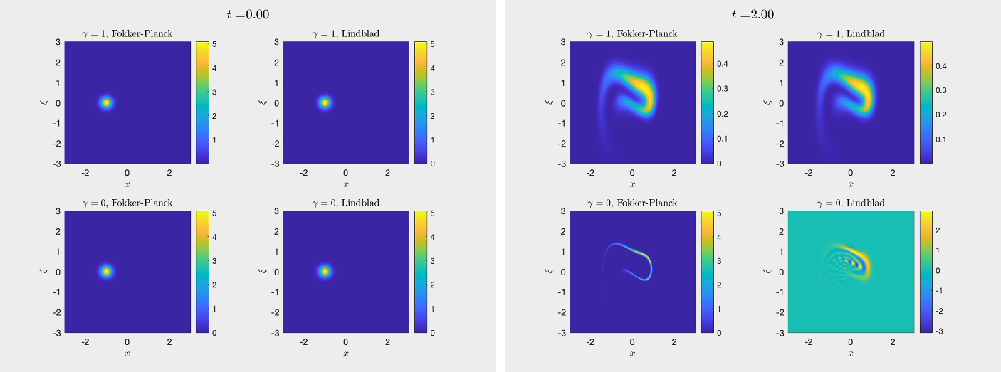
4.2 An Example

The Fokker–Planck equation can be solved explicitly when the Hamiltonian is quadratic and the Lindbladians are linear for Gaussian initial data—see for instance [10]. This gives simple examples that we can compute, and we see that in general, we cannot do better than Lemma 4.5. We consider an example in \(\mathbb ^2_\) given by

$$\begin Q = \varepsilon ^2 \Delta + x \partial _x - \xi \partial _\xi . \end$$

(4.25)

This corresponds to the jump functions \(\ell _1(x, \xi ) = x\) and \(\ell _2(x, \xi )= \xi \), and the Hamiltonian \(p(x, \xi ) = x \xi \). Consider the initial data

$$\begin u_0(x) = \frac \exp \left( -\frac \right) . \end$$

The equation preserves Gaussians as well as the symmetry about the x and \(\xi \) axis. Therefore, the solution to (3.5) must be of the form

$$\begin u(x, \xi , t) = (a(t) b(t))^}\exp \left( - \frac - \frac \right) . \end$$

Then solving for a(t) and b(t), we find

$$\begin a(t) = (h - 2 \varepsilon ^2) e^ + 2 \varepsilon ^2, \qquad b(t) = (h + 2 \varepsilon ^2) e^ - 2 \varepsilon ^2. \end$$

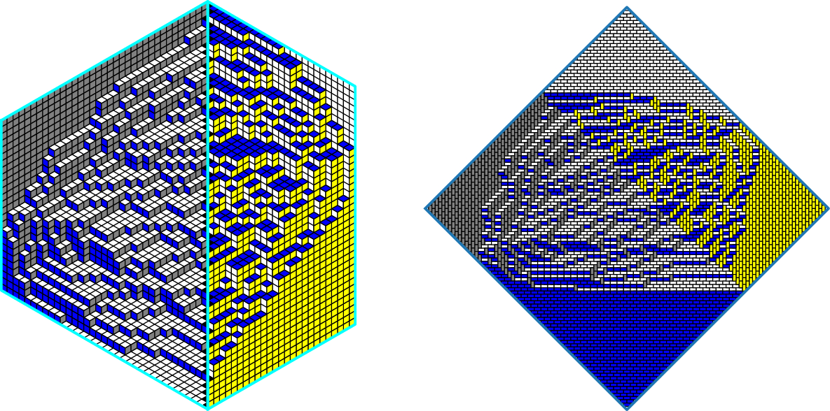
See Fig. 2.

Fig. 2

Fokker–Planck evolution of the standard coherent state centered at 0 by (4.25) in the regime \(h \le \varepsilon ^2 \le 1\)

In particular, observe that for \(t \ge 1\), u oscillates on scale \(\varepsilon \) in the x direction if \(h \le \varepsilon ^2 \le 1\) (which corresponds to the regime of Theorem 1). In terms of \(L^1\) estimates, we see that

$$\begin \Vert (\varepsilon \partial _x)^k u(x, \xi , t)\Vert _(\mathbb ^2)} = C_k \varepsilon ^k \alpha (t)^} \simeq C_k \end$$

From this example, we see that the smoothing estimate (4.5) is optimal in \(\varepsilon \) and t.