In this section, we study the following question:

$$\begin\nonumber \boxed &\text (X,L)\text \mathcal \text \\&\text \end } \end$$

We will approach this first by formulating the general idea, then formalizing it as a conjecture, and finally providing a constructive definition of the quiver \(\mathcal \) based on data of the augmentation polynomial A(x, y, u).

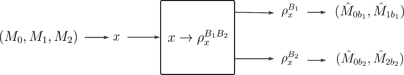
3.1 Heuristics Behind Our Proposal

BPS vortices of 3d \(}=2\) QFTs have emerged in our discussion so far as the common thread connecting various topics related to the problem addressed in this paper: from open topological strings, to symmetric quivers, to exponential networks. Following through the various connections, summarized in Fig. 8, naturally leads to the idea that, if topological strings on (X, L) admit a quiver description, then \(\mathcal \) must be encoded by the exponential network.

Fig. 8

Relations between augmentation varieties and quivers. In blue: the standard route [3,4,5,6, 9]. In red, our proposal (color figure online)

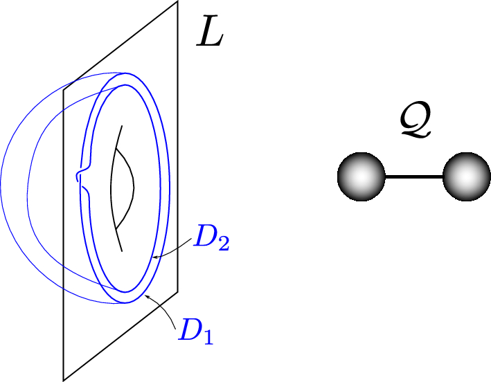
More specifically, when the open topological string partition function admits a quiver description as in (2.12), the whole BPS spectrum of M2 branes captured by LMOV invariants is generated by a finite set of basic BPS states. The basic states correspond to M2 branes wrapping holomorphic disks \(D_i\) in X with boundary on L, and their interactions are mediated by the A-brane in a way that is controlled by the linking of their boundaries (2.14). Together this data defines a quiver \(\mathcal \) with adjacency matrix

$$\begin C_ = \textrm(\partial D_i, \partial D_j)\,. \end$$

(3.1)

The 3d-3d correspondence provides a dual QFT description involving a 3d \(}=2\) QFT T[L], for which \(\mathcal \) encodes a Lagrangian description \(T[\mathcal ]\) as a \(U(1)^m\) Chern–Simons matter gauge theory. The basic M2 branes map to BPS vortices with unit charge, and the linking matrix maps to effective Chern–Simons couplings, see Fig. 4. Moreover, Chern–Simons couplings govern the dynamics of BPS vortices: in particular the orbital spin of a 2-vortex boundstate is proportional to \(\kappa _^}\), see Appendix A for a derivation

$$\begin C_ = \kappa ^}}_ \quad \leftrightarrow \quad \text \,. \end$$

(3.2)

The above chain of logic leads to the conclusion that, if one can compute all BPS vortices with unit charge of T[L], together with their spin and the spin of their boundstates, this information should encode the quiver \(\mathcal \). We propose that all this information can be extracted directly from the geometry of the augmentation variety \(\Sigma \), which arises as the moduli space of the A-brane on L in the framework of Legendrian Contact Homology [9], or equivalently as the moduli space of vacua of the 3d-3d dual theory T[L].

More specifically, exponential networks encode the BPS spectrum of kinky vortices, whose (ii, n)-sector corresponds to standard BPS vortices with vorticity n and zero Kaluza–Klein momentum.Footnote 14 Moreover, for a specific choice of vacuum i, in the limit \(x\rightarrow 0\) the spectrum of (ii, n) vortices agrees with the prediction from open topological string theory through (2.7). This settles the question of computing the BPS vortices with unit charge. Next we discuss how their spin can be computed.

The spin of BPS kinks in 2d (2, 2) QFTs is encoded by spectral networks [18], as the writhe (i.e., the algebraic self-intersection number) of the path a encoding the soliton charge

$$\begin \text = }(a) \,. \end$$

(3.3)

This definition has a natural lift to exponential networks, viewing them as spectral networks for the corresponding KK theory [11].

Observe in fact that the writhe of two concatenated open paths computes their mutual intersection

$$\begin \langle a,b\rangle = }(ab) - }(a) - }(b)\,. \end$$

(3.4)

Therefore, the intersection between (concatenatable) paths a, b measures the difference between the spin of their boundstate ab and the spin of the constituents, namely the (appropriately quantized) orbital angular momentum of the 2-vortex system

$$\begin \langle a,b\rangle = \text \,. \end$$

(3.5)

This parallels the well-known statement that the Dirac pairing, which measures the orbital angular momentum of dyons in 4d, is captured by intersections of paths on Seiberg–Witten curves [17]. This leads us to the following conjecture, illustrated in Fig. 9

Fig. 9

Left: Two solitons a, b of type (ii, 1). To compute mutual intersections (red dot), we consider the concatenation obtained by shifting b by one unit in the logarithmic label of its endpoints, as explained in Sects. 3.3–3.4. The self-intersection of a denoted by a blue dot does not contribute to the quiver matrix, since it appears both in \(}(a)\) and in \(}(ab)\) in (3.4). Right: The corresponding quiver diagram encodes the mutual intersection between \(\langle a,b^\rangle =+1\) as well as a self-intersection \(\langle a,a^\rangle =+1\) computed by concatenation of a with its own shift (color figure online)

Conjecture 1

Let \(\Sigma \) be an algebraic curve

$$\begin \Sigma = \}^*\times }^*;\ A(x,y,u) = 0\}\,. \end$$

(3.6)

where \(u = \\) is a generic set of complex moduli. Suppose that \(\Sigma = \Sigma ^\mathcal \) admits a presentation as a quiver augmentation curve as defined in (2.25). The underlying quiver structure, including vertices, adjacency matrix and fugacities (see (2.20)), can be obtained as follows.

1.

Let \(x_} \in }^*\) be a point sufficiently close to 0, and let i denote the distinguished vacuum. The spectrum of BPS kinky vortices with unit charge in vacuum i is generated by a distinguished basis of \(m = \dim \mathcal _(x_\text )\) states with CIFV index of unit norm \(|\mu _|=1\), which are in 1-1 correspondence with the vertices of \(\mathcal \)

$$\begin\nonumber \text \mathcal \ \ \leftrightarrow \ \ \text \lim _\rightarrow 0}\mathcal _(x_\text )\,. \end$$

Each basis state corresponds to a calibrated path \(a_j\) on \(\widetilde\), with \(j=1,\dots , m\), which is computed by exponential networks at the phase of its central charge \(\vartheta _j = \arg Z_\).

2.

Quiver fugacities of \(T[\mathcal ]\) are encoded by central charges computed by 1-chain integrals (2.27) on the basis paths

$$\begin c_j = \frac} \exp \left( \frac}\right) \,,\qquad j=1\dots m\,. \end$$

(3.7)

3.

The intersection matrix of the m basic paths \(\langle a_i, a_j\rangle \) coincides with the adjacency matrix \(C_\) of the quiver

$$\begin\nonumber C_ = \langle a_i, a_j\rangle \,. \end$$

This conjecture applies in particular to the computation of quivers \(\mathcal \) associated with theories T[L] arising from toric branes and knot conormals, among other examples. By viewing \(T[\mathcal ]\) as a deformation of T[L] as explained in Sect. 2.3, the quiver data for T[L] is obtained by specializing to the limit \(c_i \rightarrow Q^\). That is, applying our conjecture directly to the augmentation curve A(x, y, Q), the quiver can be obtained from exponential networks.

3.2 Algorithm

To complement and sharpen our main conjecture, we next explain how the data of the quiver should be computed from an algebraic curve in \((}^*)^2\). Here we summarize the algorithm, and later we will develop each point in more detail.

1.

Fix a suitable choice for the theory point, i.e., a point \(x_\text \in }^*_x\),Footnote 15 in such a way that the spectrum of (ii, 1) BPS kinky vortices for the distinguished vacuum i is stabilized under wall-crossing (2.6). Concretely, this implies choosing \(x_\text \) sufficiently close to 0, as demonstrated in [16].

2.

Compute the spectrum of (ii, 1) kinky vortices using exponential networks, by keeping track of all network trajectories of type (ii, 1) that swipe across \(x_\text \) as \(\vartheta \) varies in \([-\pi ,0)\). Denoting the corresponding soliton paths (a precise definition is given below) by \(a_k\) for \(k=1,\dots , m\), each is associated with a vertex of \(\mathcal \).

3.

The central charge of each soliton admits a decomposition

$$\begin Z_ = 2\pi i \left[ \log x_\text + \sum _s (\beta _k)_s \, \log u_s\right] \,, \end$$

(3.8)

in terms of integers \((\beta _k)_s\), which are the data that defines the classical limit (i.e., \(q=1\)) of quiver fugacities \(x_k\) in (2.12)

$$\begin c_k = \prod _s ^\,. \end$$

(3.9)

4.

The intersection matrix of (ii, 1) soliton paths, defined by path concatenation as in (3.4), determines the quiver adjacency matrix:

$$\begin C_ = \langle a_k , a_l \rangle \,. \end$$

(3.10)

The implementation of each step involves certain subtleties, which we address next.

3.3 Quiver Vertices and Fugacities

We begin by discussing the steps that give the vertices of \(\mathcal \) and the associated fugacities \(c_i\).

3.3.1 Identification of kinky vortex charges with paths on \(\widetilde\)

We recall some details regarding the definition of charges of kinky vortices in terms of 1-chains on \(\widetilde\); more details can be found in [11, 16].

Given \(\Sigma \) as in (3.6), we view it as a (possibly ramified) covering of \(}^*_x\), with sheets given locally by the roots \(y_j(x)\) for \(j=1,\dots , K\). We further introduce a logarithmic covering \(\widetilde\) of \(\Sigma \) branched at punctures corresponding to \(y=0,\infty \), with sheets \(\log y_j(x) +2\pi i \, N\) labeled by \(N\in }\). A choice of trivialization for these coverings, i.e., a system of branch cuts and a globally defined labeling (j, N) of sheets of \(\widetilde\) as a covering of \(}^*_x\), will be understood from now on.

Charges of kinky vortices, or solitons, are classified by relative homology classes of paths on \(\widetilde\) interpolating between vacua (i, N) and \((j,N+n)\). We label soliton charges only by the flux n that they carry, and not by the logarithmic label N of the vacuum they start from, since only the difference is physically observable due to the overall shift symmetry \(N\rightarrow N+1\) arising from large gauge transformations on \(S^1\times }^2\). The action of large gauge transformations on soliton paths is implemented by a shift map constructed in [11]. Consider a class of paths \(a^\), with \(N\in }\), interpolating respectively between vacua

$$\begin \textrm(a^) = (i,N)\,, \qquad \textrm(a^) = (j,N+n)\,, \end$$

(3.11)

where (i, N) denotes the point \((x, \log y_j(x)+2\pi i N)\in \widetilde\). They have the same CFIV indices and central charges if and only if they are related by the shift map,Footnote 16 and in this case, we identify them as charges

$$\begin \mu _} = \mu _}\,, \quad Z_} = Z_} \qquad \Rightarrow \qquad a^\sim a^\,. \end$$

(3.12)

We denote the equivalence class of paths simply as a, omitting the index N. When it will be important to discuss the choice of a representative, we will sometimes denote by a the representative \(a^\) and its shifted copies by \(a^\).

3.3.2 Fixing the theory point by stabilization of the (ii, 1) sector

The BPS spectrum of kinky vortices, i.e., the collection \(\\) of CFIV indices and central charges for all soliton charges a, depends on a choice of \(x\in }^*\) due to wall-crossing phenomena in the parameter space of couplings of the 3d \(}=2\) QFT, for which x plays the role of a (complexified and exponentiated) Fayet-Ilioupoulos coupling.

The spectrum jumps when x crosses lines of marginal stability, whose definition is

$$\begin }(a,b) = \}^*; \mu (a) \mu (b) \ne 0, \ Z_a / Z_b\in }_,\ \mathrm =\textrm(b)\}\,. \end$$

(3.13)

In other words, MS walls of two solitons a, b are loci in \(}^*\) where both states have nonzero CFIV index, their central charges have the same phase, and solitons can be concatenated so that the vacuum corresponding to the end of a coincides with the vacuum corresponding to the beginning of b.

In general, \(\textrm(a,b)\ne \textrm(b,a)\) due to concatenation ordering. A soliton of type (ij, n) i.e. interpolating between vacuum (i, N) and \((j,N+n)\) can only be concatenated with a soliton of type (jk, m), for arbitrary \(k\in 1,\dots , K\) and \(m\in }\). An important exception occurs for solitons of types (ii, n): if both a, b are of this type, then concatenation is possible with both orderings and \(}(a,b)=}(b,a)\).

The structure of MS walls for kinky vortices of type (ii, n) has been studied extensively in [16]. As x approaches 0, the central charge of (ii, n) solitons is dominated by:

$$\begin \lim _ Z_a = \frac\int _a\log y \, d\log x \approx n \log x +\dots \end$$

(3.14)

On the other hand, the pattern of CFIV indices is typically rather intricate, due to an infinite sequence of MS walls that are located near 0. Denoting by \(}_\) all marginal stability walls where (ii, n) solitons can be generated

$$\begin }_ = \bigcup _ }(a,b)\,, \end$$

(3.15)

we observed that these are all contained in an annular region of finite size around \(x=0\)

$$\begin r^-_< \}_\} < r^+_\,. \end$$

(3.16)

Therefore, the CFIV index of a soliton a of type (ii, n) will undergo a sequence of transitions, but will eventually stabilize once \(|x_\text | < r_^-\). We denote the stabilized spectrum by \(\mu _a\)

$$\begin \mu _a := \mu _a(x) \quad \forall |x|<r_^-\,. \end$$

(3.17)

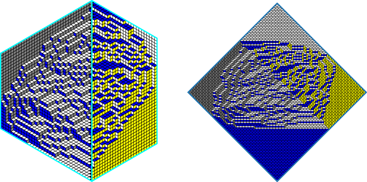
The spectrum of stabilized kinky vortices is expected to agree with the spectrum of standard BPS vortices, with a suitable identification of their partition functions [16]. An example is shown in Fig. 10. For the purpose of computing quivers from augmentation curves, we will only be interested in the stabilized spectrum of (ii, 1) solitons.

Fig. 10

Walls of marginal stability and stabilized and unstabilised theory points for (ii, 1) solitons on \(}^*_x\) in the theory described by the mirror of \(\mathbb ^3\), see [16, 47] for more details (color figure online)

3.3.3 Computation of the stabilized spectrum

Having fixed a suitable theory point, the next task is to compute the stabilized spectrum of (ii, 1) kinky vortices. This can be achieved by a standard application of exponential networks, see in particular [11] for details on the computation of CFIV indices. Given \(\Sigma \), the exponential network \(\mathcal (\vartheta )\) is a web of trajectories on \(}^*_x\) corresponding to solutions of the BPS soliton equations, whose geometric counterpart is the ODE

$$\begin (\log y_j - \log y_i +2\pi i \, n) \frac = e^\,. \end$$

(3.18)

The equation is integrated starting from branch points \(y_i(x)=y_j(x)\), or from punctures where \(|\log y(x)| \rightarrow \infty \), or from intersections of trajectories. The shape of the network depends on \(\vartheta \).

Kinky vortices for the QFT whose FI coupling is \(x_\text \) are encoded by trajectories of \(\mathcal \) that pass through \(x_\text \) for any value of \(\vartheta \). In fact, if the BPS spectrum contains a kinky vortex with charge a, then there will be a trajectory of \(\mathcal \) that passes through \(x_\text \) exactly when the phase is that of its central charge

$$\begin \vartheta _a := \arg Z_a(x_\text ) \,. \end$$

(3.19)

Recall that \(Z_a\) is a 1-chain integral (2.27) on \(\widetilde\). The class of models considered in this paper, which includes toric branes of toric CY3 with \(b_4=0\) and knot conormal branes in the resolved conifold, has the special property that any closed periods of \(\widetilde\) are linear combinations of complex moduli

$$\begin Z_ = 2\pi i \sum _s k_ \, \log u_s\,,\qquad k_\in }\,. \end$$

(3.20)

Focusing on (ii, n) BPS states, and given their physical interpretation as vortices with unit flux on the cylinder [16], it follows that their central charge is determined by a collection of integers \(k_\)

$$\begin a \text (ii,n) \quad \Rightarrow \quad Z_ = 2\pi i \left[ n\log x_\text + \sum _s k_ \, \log u_s\right] \,. \end$$

(3.21)

Fig. 11

An (ii, 1) soliton web from the exponential network for the mirror curve of the resolved conifold, see Sect. 4.2. The orange cross is a branch point, the dashed orange line is a polynomial branch cut, the black dot is the puncture, the black dashed line is a logarithmic branch cut, the orange point is the theory point and the solid lines are the relevant trajectories. Although not shown here, we will use a black cross for logarithmic branch points away from punctures (color figure online)

Solitons of type (ii, n) are carried by trajectories of the same type, which can be generated either at punctures with \(|\log y|\rightarrow \infty \), or at intersections of other trajectories (but not at branch points). In either case, a calibrated path on \(\widetilde\) of class a is obtained by lifting to appropriate sheets of \(\widetilde\) the trajectories that underlie the soliton: this includes the (ii, n) trajectory, but also any of its parents, see Fig. 11a for an example.Footnote 17 The lift involves taking two copies of an (ij, n) trajectory to sheets (i, N) and \((j,N+n)\) with opposite orientations. The choice of N is irrelevant as discussed earlier.

Since an exponential network \(\mathcal (\vartheta )\) includes the CFIV index of each path \(\mu _a\) as part of its data, by scanning over all phases \(\vartheta \), and keeping track of trajectories that sweep across \(x_\text \), the entire spectrum of kinky vortices at \(x_\text \) can be obtained. Computing the spectrum for a value of \(x_\text \) for which \(\mathcal _\) is stabilized ensures that we detect all states corresponding to kinky vortices with unit vorticity \(n=1\). Let \(a_\) with \(k=1,\dots , m\) denote the (equivalence classes) of calibrated paths of type (ii, 1) computed by the exponential network, we define a set of vertices of the quiver \(\mathcal \) in 1-1 correspondence with \(\_^m\). The fugacities \(c_i\) associated with vertices of \(\mathcal \) are defined by the decomposition of the central charges \(Z_\) given in (3.8)–(3.9).

Remark 1

(Uniqueness of \(a_k\)) The exponential network \(\mathcal \) computes the spectrum \(\,\mu _\}_^\) and additionally determines calibrated paths on \(\widetilde\) in class \(a_k\) for each of the (ii, 1) basis states. However, there may be more than one calibrated path for a given charge \(a_k\). This is because the CFIV index is integer-valued and soliton-anti-soliton pairs can give rise to cancelations. Since our algorithm for building \(\mathcal \) requires us to determine a unique path for each \(a_k\), it is essential to address how to deal with the possibility of cancelations. We will argue how to do this by a deformation argument.

First we observe that \(|\mu _|=1\) is necessarily true, because of the following reason. Suppose that \(\Sigma \) admits a quiver description \(\Sigma ^\mathcal \). Then it is possible to write it as an algebraic curve \(A(x,y,c_1,\dots , c_m)=0\) and by taking \(c_j\rightarrow 0\) except for a distinguished value of j, turns the curve into \(1-y-c_j (-y)^} x=0\), as it follows from (2.24) that all other \(y_\rightarrow 1\) in this limit. Then, the resulting curve corresponds to the mirror of \(}^3\), which was analyzed in [16], where it was shown that there is a unique (ii, 1) kinky vortex close to \(x=0\), with \(\mu _a=\pm 1\).

Next, we can turn back on the other \(c_\ne 0\) up to the original values that determine \(\Sigma \) as a specialization of \(\Sigma ^\mathcal \). In this process, it may happen that new stable solitons arise in the charge sector \(a_j\), but by invariance of the CFIV index these must come in particle-antiparticle pair. Keeping track of these, we can distinguish the original soliton from the canceling pairs and select a unique calibrated path in class \(a_k\). We will see an example of this in Sect. C.

3.4 The Adjacency Matrix

The computation of \(C_\) from intersections of open paths as defined in (3.4) involves several delicate steps:

A soliton charge a corresponds to an equivalence class of (relative homology classes) paths on \(\widetilde\) established by the shift map (3.12). To define the class of the concatenation of two paths \(a_j\), \(a_k\), it is necessary to choose compatible representatives \(a_j^, a_k^\), which admit a concatenation. If follows from definitions that the equivalence class (under shift map) of the latter is independent of the choice of representatives.

To define a smooth concatenation, it is necessary to choose a capping path that connects smoothly the endpoint of the first path to the starting point of the second one. This choice is a priori non-canonical and must be considered as part of the definition of the intersection pairing.

An additional subtlety that arises with (ii, 1) paths is that both \(a_j a_k\) and \(a_k a_j\) are valid concatenations. This raises the question of whether the intersection pairing is symmetric under exchange \(\langle a_j,a_k\rangle = \langle a_k, a_j\rangle \), which is needed for consistency with the symmetry of the quiver’s adjacency matrix.

3.4.1 Resolution of projected soliton paths

While paths are defined on \(\widetilde\), having chosen a trivialization with global labels (j, N) for its sheets over \(}^*_x\), it will be convenient to work with projections of the soliton paths to the base. The projection is, however, degenerate, and to compute intersections it will be useful to adopt a choice of resolution.

As shown in Fig. 11a, a soliton path in class \(a_k\) is associated with a collection of trajectories in \(\mathcal \), which we call the soliton web of \(a_k\) and which we denote by \(a_k^}\). The soliton web coincides, in fact, with the projection of \(a_k\) down to \(}^*_x\) (possibly with multiplicities attached to each of its edges). Therefore to define a resolution of the projection of \(a_k\), it is sufficient to define a resolution of the associated soliton web.

Let a be the charge of a kinky soliton of type (ii, 1). Its projection to \(}^*_x\) consists of a collection of arcs on \(}^*_x\) obtained by taking, for each trajectory of type (jk, n) in the soliton web \(a^\mathcal \), a copy labeled by (j, N) and a copy labeled by \((k,N+n)\) oriented, respectively, anti-parallel and parallel to the trajectory itself.Footnote 18 The label N associated to each arc is determined by compatibility with gluing at junctions with other arcs, as determined by a choice of representative for a itself.

A resolution of the soliton web \(a^}\) is then given by a choice of capping paths to glue the above collection of arcs on \(}^*_x\), according to the following rules:

1.

Away from branch points, the \((j,n+N)\)-labeled arc is on the right side, while the (k, N)-labeled arc is on the left side of the trajectory, viewed with respect to the direction of increasing t in (3.18).

2.

Around polynomial branch points, the computation of intersection number involves choosing a resolution for the projection of soliton paths. This presents a potential source of ambiguity because the resolution of each path can turn either clockwise or counterclockwise around a quadratic branch point. In Appendix B.1, we show that the intersection number is, however, invariant. For higher-order polynomial branch points, the choice of resolution is dictated by the monodromy itself, and no such ambiguity is present.

3.

At junctions of trajectories of types (ij, n), (jk, m) and \((ik,m+n)\), the resolution of soliton paths involves smoothing cusps. The choice of smoothing can introduce extra intersections (kinks) in the path; however, these drop out of the mutual intersection number defined via (3.4). Therefore, any choice of smoothing can be used. For simplicity, we will adopt the choice that does not involve additional kinks.

4.

At a logarithmic branch point, the projected soliton paths can be smoothed in such a way that it turns either clockwise or counterclockwise around the branch point. The choice is uniquely fixed by the signature of the logarithmic shift around the branch point, see Appendix B.1.

An example is shown in Fig. 11b.

3.4.2 Concatenation

Next we define the concatenation of paths of type (ii, 1) by using their resolved projections. Naturally, the concatenation takes place at \(x_\text \) where both resolved paths have their endpoints. However, the issue that we need to solve is that the tangents at the endpoints of the paths to be concatenated typically do not match. Therefore, additional arcs need to be introduced to define a concatenation.

The tangent of a projected soliton at its endpoint \(x_\text \) depends on the phase \(\vartheta _a\) of its central charge (3.19). In fact, solutions of (3.18) for (ii, n) solitons are actually independent of i and n (up to rescaling of t) and are spirals given by

$$\begin x(t) = x_} e^ (t-t_0)}}\,. \end$$

(3.22)

Note that requiring \(\lim _x(t) = 0\) implies that \(\vartheta _ \in [-\pi , 0]\) for all \(j = 1,2,\dots , m\).Footnote 19 Due to this, the angle between the two trajectories will be acute, and further looking at the slopes of the (ii, 1) trajectory at the theory point using Eq.  (3.22)

$$\begin x'(t_0) = \frac e^}}\,, \end$$

(3.23)

we conclude that the phase \(\vartheta _\) of the translucent green trajectory corresponding to the projection of \(a_j\) is less than that of the pink trajectory \(\vartheta _\) in Fig. 12.

Moving on to the actual concatenation, we start by recalling that to concatenate two (ii, 1) soliton paths, both the polynomial and logarithmic branches of the end of the first soliton path should match with that of the beginning of the second soliton path. Assuming that the phases of the two solitons are different, the redundancy in choosing the base logarithmic branch gives us two distinct possible concatenations, which we show in Fig. 12.

As it turns out, the correct choice for recovering the quiver is counterclockwise concatenation, which according to above also imposes the decreasing phase ordering of concatenation among projected paths. Therefore, we define the concatenation of two paths of type (ii, 1) as follows (oriented from left to right)Footnote 20

$$\begin a_ a_ \quad \text \vartheta _< \vartheta _\,. \end$$

(3.24)

Fig. 12

Zoomed in near \(x_\text \), the translucent green and pink trajectories belong two different (ii, 1) soliton webs, with their base logarithmic indices chosen so that concatenation of soliton paths is possible. As mentioned in the text, the counterclockwise concatenation is the correct choice for obtaining the quiver (color figure online)

The above rule does not address the case of paths with the same phase. This situation can happen in two distinct cases: either in the computation of the self-intersection number, when one studies the concatenation of a soliton path with a (shifted, as in (3.12)) copy of itself, or when moduli of \(\Sigma \) are not generic. In these cases, both choices for the ordering of concatenation give the same intersection pairing. More details on these cases will be given in actual examples and further in Appendix B.2.

3.4.3 The intersection pairing matrix

The intersection of two paths \(\langle a,b\rangle \) is defined by (3.4), where the write of each path and of their concatenation is obtained by counting double points in the resolved soliton webs \(a^}, b^}\) and \(ab^}\) defined by choosing appropriate capping paths as explained above. Each double point of arcs with coincident labels \((j,N) = (j',N')\) contributes \(\pm 1\) according to the rule given in Fig. 13

$$\begin }(a) = \sum _} \pm 1\,. \end$$

(3.25)

This convention is adapted to recover quiver adjacency matrices in examples discussed below.

Fig. 13

Intersection numbers accord