Inferring the cell state dynamic relationships

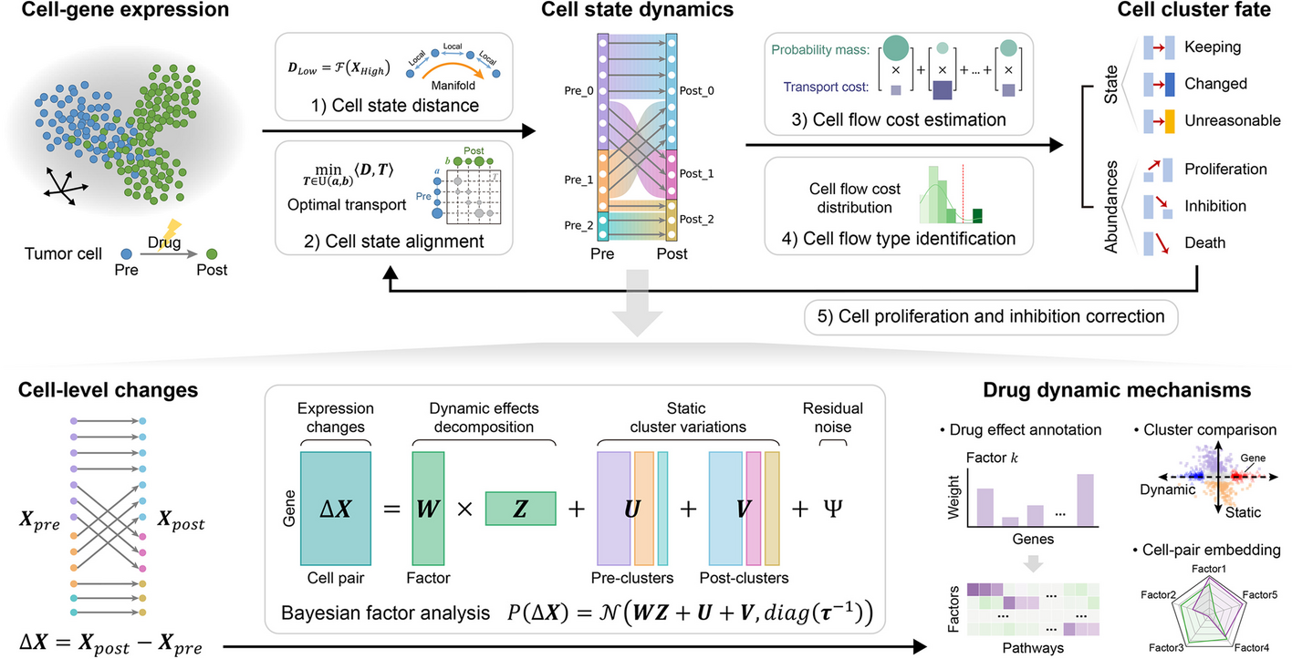
To characterize the cell states in a high-dimensional gene expression space and identify their alignment relationships, we designed the following computational steps in scStateDynamics.

Identifying cell states and estimating their transcriptomic profiles

Due to the stochastic nature of gene transcription and the limited detection capacity for rare transcripts, scRNA-seq data often exhibit high-frequency dropout events, resulting in a large proportion of zeros in the gene expression matrix (Additional file 1: Fig. S15) [54,55,56]. To mitigate the influence of dropout event noise, we add a preprocessing step of grouping several similar cells into a metacell to represent a type of cell state [57,58,59]. In practice, we utilize the “Scanpy” package [60] to perform clustering with a large ‘resolution’ parameter setting (such as 30 or 50). Each resulting cluster is considered as a metacell, generally consisting of approximately three to ten cells, to represent a specific cell state. This adaptive numbers of cells within metacells can better cope with the varying densities of cell distribution in gene expression space. Then, we characterize each metacell by calculating the average expression profiles of its constituent cells. Generally, the cells with very similar expression profiles can be seen as being resampled from a common cell state, and the probability of dropout events occurring simultaneously in these similar cells for a given gene is relatively low. Therefore, this preprocessing step of aggregating similar cells and utilizing their average expression values to represent the corresponding cell states can reduce the dropout noise. The analysis on our testing datasets also validated its necessity and effectiveness (Additional file 1: Fig. S15), thereby a meta-cell can also be regard as a denoised representation of a cell. Besides, it can reduce the computational complexity of subsequent analyses. Notably, to make this preprocessing step more flexible and robust, we provide an interface for users to either supply their own metacell labels or bypass this preprocessing step through setting unique metacell labels.

Measuring the distances between cell states along the low-dimensional manifold

In the high-dimensional gene expression space, cells are usually distributed on a low-dimensional manifold. This observation suggests that direct calculation of global Euclidean distances may not provide an accurate representation of the similarities between cells along the manifold. Hence, we refer to the methodologies of PHATE [21], Diffusion Map [20], and MuTrans [15] algorithms and utilize local distance diffusion to assess the global relationships among different cell states. In detail, we use the Gaussian kernel function \(}}_\left(x,y\right)=\text\left(-\frac}}_-}}_\Vert }^}\right)\) to transform the global Euclidean distances between the joint-embedded expression profiles \(}}_\) and \(}}_\) of metacells \(x\) and \(y\) into local affinities. This transformation ensures that the affinity degree between two cell states is greater than 0 only when they are close enough, so that we can obtain the local neighbor relationships based on the affinity degrees (Additional file 1: Fig. S16a). The parameter \(\epsilon\) governs the local bandwidth constrained by the kernel function (Additional file 1: Fig. S16b). Considering that the density of the cell distribution is uneven, the k-nearest-neighbor distance \(_\left(x\right)\) is used as an adaptive bandwidth. Additionally, to control the heavy tail of the Gaussian kernel when \(_\left(x\right)\) is large, the exponent \(\alpha\) is introduced (Additional file 1: Fig. S16b). Consequently, the resulting kernel function is obtained by taking the average of two kernel values to ensure the symmetry of the affinity matrix: \(}}_\left(x,y\right)=\frac\text\left(-}}_-}}_\Vert }^}_\left(x\right)}\right)}^\right)+\frac\text\left(-}}_-}}_\Vert }^}_\left(y\right)}\right)}^\right)\). Then we normalize the affinity matrix by its row sums to generate the following random-walk transition probability matrix among cell states \(}\left(x,y\right)=\frac}}_\left(x,y\right)}_}}_\left(x,z\right)}\). Furthermore, to propagate the local neighbor relationships and assess the long-range affinity values along the low-dimensional manifold, we perform a \(t\)-step random walk and calculate the \(t\)-step diffusion probability \(}}^=}}^}\). Here, the parameter \(t\) is a positive integer that denotes how many steps of long-range diffusion are considered acceptable, and it can be determined based to the distribution density of cells. And \(}}^\) is an identity matrix. Finally, we measure the distance between two cell states by calculating the \(^\)-norm distance of their logarithmic \(t\)-step diffusion probabilities to other cell states: \(}}_=\sqrt\left(}}_^\right)-\text\left(}}_^\right)\Vert }^}\). Notably, at this distance measurement step, we assume that the influence of batch effects on measuring distances between cells along the manifold is slight. In the practice, we advise users to evaluate the extent of batch effect noise using approaches such as low-dimensional co-projection, or quantitative indicators and then determine whether and how to correct the batch effect before utilizing our algorithm. If the batch effect noise is pronounced, it is essential to correct it beforehand.

Aligning the cell states between two time points

Here, we assume that the overall changes in cell states is relatively small during drug treatment and only a portion of cells have significant state changes. Using the distances along manifold calculated above to measure the extent of cell state changes, we adopt the principle of minimizing the overall changes to align cells in a low-dimensional manifold between two time points, which can be achieved by the optimal transport algorithm. At each time point, all cells form a discrete cell state probability distribution in gene expression space. Therefore, aligning the cell states can be regarded as seeking a transport plan between two probability distributions.

In the discrete case, given the source and target probability distributions

\(}\in }_^_} \left(_^_}}}_=1\right)\) and \(}\in }_^_} \left(_^_}}}_=1\right)\)

and a \(_\times _\) transport cost matrix \(}\in }_^_\times _}\), where each element \(}}_\) indicates the cost when transporting from state \(i\) to \(j\). Then, the objective of the optimal transport problem is to find a transport matrix \(}\in }_^_\times _}\) that minimizes the total cost (overall changes)

\(\langle },}\rangle =_}}_}}_\) subject to \(_^_}}}_=}}_\) and \(_^_}}}_=}}_\)

where \(}}_\) indicates the identified probability mass transporting from \(i\) to \(j\). This means that the total cost is the inner product of the cost matrix \(}\) and the transport matrix \(}\), while ensuring that the row sum and column sum of \(}\) are equal to \(}\) and \(}\), respectively.

In our cell state alignment problem, the number of cells in all metacells (cell states) at the pre- and post- time points can be normalized as probability distributions \(}\) and \(}\), respectively. Taking the distances calculated above (matrix \(}\)) as the cost matrix \(}\), we can obtain the transport matrix \(}\) based on the optimal transport algorithm, in which each element \(}}_\) indicates the probability mass transforming from the pre-timepoint to the post-timepoint. According to these transport probabilities, we can align the cells in all metacells between the two time points. This step is implemented with the “ot” Python package [61].

Grouping the cell alignment relationships into subcluster flows

To investigate the dynamics at cluster level, we conduct clustering on the cells at each time point individually using “Scanpy” package [60], with a small “resolution” parameter setting (Additional file 1: Fig. S1a). This step of separate clustering, rather than joint clustering, can avoid the influence of batch effect noise. In this way, we connect the clusters between two time points based on cell flows and identify distinct fates among cells. According to the cell fates (which post-cluster the cell transition to), we further divide the pre-clusters into distinct subclusters (Additional file 1: Fig. S1b). This operation of identifying cell subcluster flows can help infer the distinct proliferation or inhibition rates of clusters and support the subsequent differential expression analysis to dissect intra-cluster intrinsic and acquired heterogeneity between distinct cell fates.

Quantifying the dynamic characteristics of cell populations

After drug treatment, distinct clusters of tumor cells may exhibit varying degrees of sensitivity, leading to differences in proliferation or inhibition rates. Besides, some cells can also change their states to adapt to the external environment. Hence, the dynamic characteristics of cell populations include the changes in both cell states and abundances (proportions). The extent of changes in cell states can be quantified by the transport costs. However, for the cell abundances, the classical optimal transport theory we used could not model the increase or decrease in probability mass that reflects the relative proliferation or inhibition of cell populations. To address this limitation, we first identify the unreasonable cell subcluster flows caused by the neglect of cell proliferation and then correct them to obtain more reliable cell dynamics.

Identifying the types of cell subcluster flows

To quantify the extent of changes in cell states and distinguish the pattern of cell subcluster flows, we calculate the average transport cost for each flow. Given that the metacell sets at pre-timepoint \(s\) and post-timepoint \(t\) of a cell subcluster flow are \(_\) and \(_\), we define the average weighted transport cost of it as

$$\text\left(_,_\right)=\frac__,j\in _}}}_*}}_}__,j\in _}}}_}$$

According to the distribution of average transport costs of all subcluster flows, we think they can be categorized into either state-keeping, state-changed, or unreasonable flows. State-keeping corresponds to the cells that maintain high similarity, resulting in flows with low transport costs. State-changed indicates that cells adaptively adjust their states, leading to flows with relatively high transport costs. Unreasonable flows refer to some incorrect alignments identified by OT algorithm arising from the neglect of distinct proliferation or inhibition rates among cell clusters. As a result, when certain source cell populations are inhibited, their reduced probability masses have to be allocated to other target cell populations exhibiting high proliferation rates. These incorrect alignments lead to some unreasonable flows with abnormally large transport costs. To determine the type of flows, an analysis of the average transport cost distribution for all subcluster flows is conducted through plotting a histogram. If the distribution exhibits a distinct trimodal pattern, a Gaussian mixture model (GMM) can be applied to category the three peaks into state-keeping, state-changed, or unreasonable flows. Instead, if there are several outliers that are clearly distant from the majority of data points, outlier detection approaches (e.g., using 1.5 times the interquartile range above the third quartile as a threshold) can be employed to identify these outliers as unreasonable flow. Besides, manually setting the thresholds to identify unreasonable flows is also optional.

Correcting the unreasonable cell flows

Based on the identified type of cell flows, we aim to correct the unreasonable flows and estimate the proliferation or inhibition rates of clusters.

Given an unreasonable flow with a probability mass of \(\delta\) from a subset of cluster Pre_A at pre-timepoint to a subset of cluster Post_B at post-timepoint, we can infer that the cluster Pre_A is inhibited, and the inhibition rate can be calculated by dividing \(\delta\) by the total probability masses of cluster Pre_A. Meanwhile, the cluster Post_B should originate from the cells that are more similar to it. Hence, if there are other reasonable sources (without loss of generality, we refer to them as Pre_C and Pre_D) for Post_B, we assign the probability mass \(\delta\) to Pre_C and Pre_D based on their relative fractions. If Post_B completely originates from Pre_A, we think the cluster with the highest similarity to Post_B should have a greater proliferation rate. In this way, the probability masses of unreasonable flows can be assigned to more appropriate source clusters. By re-normalizing the probability masses at the pre-timepoint, we obtain the updated source probability distribution, denoted as \(}\boldsymbol}\). Then, we replace \(}\) with \(}\) to re-perform optimal transport and re-correct the identified unreasonable flows iteratively, until no outlier flows exist or the results stabilize.

In the end, by comparing the final updated source probability distribution with the initial source distribution \(}\), we can estimate the final proliferation or inhibition rate of each cluster at pre-timepoint.

Decomposing the expression changes into static variations and dynamic biological effects

The changes in gene expression profiles between the cells at two time points can provide insights into the dynamic biological mechanisms of drug action. According to the obtained optimal transport matrix \(}\), an element \(}}_\) greater than 0 indicates a potential dynamic alignment between the \(i\) th cell state (metacell) at the pre-timepoint and the \(j\) th cell state at the post-timepoint. Consequently, assuming that there are \(M\) elements greater than 0 in \(}\), we identify \(M\) alignment relationships among cell states, resulting in the formation of \(M\) distinct cell pairs. Subsequently, according to the coordinates of these \(M\) elements in \(}\), we can extract the corresponding \(M\) gene expression vectors at the pre- and post-timepoints. These vectors collectively compose the matrices \(}}^)}\in }_^\) and \(}}^)}\in }_^\), where \(G\) denotes the number of genes. Then the matrix of gene expression changes \(\Delta }\in }^\) can be calculated by \(}}^)}-}}^\right)}\). Here, we think these dynamic changes are determined by two types of effects: (i) the initial and final cell expression profiles and (ii) the molecular mechanisms of drug action. To disentangle these two types of variations, we design a Bayesian factor analysis model by characterizing the first type of static variations with the cell cluster identities and decomposing the second type of dynamic effects into a combination of gene factors (signatures).

Model representation

Assuming that there are \(S\) and \(T\) clusters at the two time points, then for a cell pair \(m\in \left\,\dots ,M\right\}\), consisting of a metacell within cluster \(s \in \left\,\dots ,S\right\}\) and a metacell within cluster \(t \in \left\,\dots ,T\right\}\), we decompose its change vector \(\Delta }}_\) into a sum of three components and an additive Gaussian noise:

$$\Delta }}_=}}_+}}_+}}}_+}$$

Here, vector \(}}_\in }^\) denotes the common effects shared by the cells in cluster \(s\) at pre-timepoint, while vector \(}}_\in }^\) denotes the effects shared by the cells in cluster \(t\) at post-timepoint. We model them with normal distributions

$$P\left(}}_\right)=\mathcal\left(\mathbf,_^\mathbf\right)$$

$$P\left(}}_\right)=\mathcal\left(\mathbf,_^\mathbf\right)$$

The matrix \(}\in }_^\) denotes the regulatory weights of \(K\) factors on genes, and each factor can be seen as a gene signature related to the dynamic biological mechanism of drug action. We constrain the elements in it to be positive and use independent log-normal distribution to model it

$$P\left(}\right)=_^\text\left(\mathbf,_^\mathbf\right)$$

The vector \(}}_\in }^\) denotes the composition coefficients (activities) of the factors for cell pair \(m\), and can also be seen as an embedding of this cell pair in the space spanning by these gene factors. We model it with normal distribution

$$P\left(}}_\right)=\mathcal\left(\mathbf, _^\mathbf\right)$$

The vector \(}\in }^\) is Gaussian residual noise

$$P\left(}\right)=\mathcal\left(\mathbf, diag\left(}}^\right)\right)$$

We use the precision parameter \(}}_\) to capture the gene-specific variation and define an independent conjugate prior for it

$$P\left(}\right)=_^\text\left(_,_\right)$$

In these distributions, \(_\), \(_\), \(_\), \(_\), \(_\), and \(_\) are hyperparameters \(.\)

Hence, we can imply the likelihood as

$$P\left(\Delta }\boldsymbol|\boldsymbol},},},},}\right) = _^\mathcal\left(\Delta }}_\boldsymbol|\boldsymbol}}}_+}}_+}}_, diag\left(}}^\right)\right)$$

Inference

Given the observation variable \(\Delta }\), the latent variables \(}\), \(}\), \(}\), \(}\), and \(}\) are not mutually independent. Exact inference for the posterior distribution \(P\left(},}, },},}\boldsymbol|\Delta }\right)\) requires integrals, which are computationally intractable. Hence, we use the strategy of variational inference to approximate the true posterior distributions. We introduce a parameterized variational distribution \(_\left(},}, },},}\right)\), which can be factorized as

$$_\left(},}, },},}\boldsymbol\right)=_\left(}\right)_\left(}\right)_\left(}\right)_\left(}\right)_\left(}\right)$$

where \(\phi\) are all the variational parameters in each of the following distributions

$$_\left(}\right)=\prod_^\prod_^\text\left(__},__}^\right)$$

$$_\left(}\right)=\prod_^\prod_^\mathcal\left(__},__}^\right)$$

$$_\left(}\right)=\prod_^\prod_^\mathcal\left(__},__}^\right)$$

$$_\left(}\right)=\prod_^\prod_^\mathcal\left(__},__}^\right)$$

$$_\left(}\right)=\prod_^\text\left(_,_\right)$$

Hence, our goal is to optimize the parameters \(\phi\) to find the best possible variational distribution \(_\) that effectively approximates the posterior distribution. When we use Kullback–Leibler divergence \(\text\left(_\left(},}, },},}\boldsymbol\right) | P\left(},},},},}\boldsymbol|\boldsymbol\Delta }\right)\right)\) to measure the distance between these two probability distributions, the optimization problem can be converted to maximize the evidence lower bound (ELBO)

$$\text=}__}\left[\textP\left(\Delta },\boldsymbol},},},},}\right)-\text_\left(},}, },},}\right)\right]$$

The optimization and update of variational parameters \(\phi\) are performed by using stochastic gradient descent algorithm (Adam optimizer).

Datasets and pre-processingSimulated data generation

To evaluate the performance of scStateDynamics, we used the “paths” method of the “splatSimulate” function within the Splatter package [22] to generate three scRNA-seq datasets that simulate distinct scenarios of tumor drug responses. To design the characteristics of these dynamic processes, we mainly manipulated the following parameters. We used the “group.prob” to control the sizes of cell clusters and used the “path.from” parameter to determine the dynamic relationships between clusters. Then, to model the extent of changes in cell states, we adjusted the “de.prob” parameter. Besides, we utilized the “path.skew” parameter to fine-tune the distribution of cells towards either the source or target population.

Data pre-processing

The pre-processing for the simulated and real data was performed based on the Scanpy [60], Seurat [62], and scCancer [63, 64] packages. First, data quality control is performed by filtering the potential lysed cells, low-quality cells, and doublets, based on the number of detected transcripts and genes, as well as the percentage of transcripts from mitochondrial genes. Besides, mitochondrial genes, ribosomal genes, and the genes expressed in fewer than three cells are also filtered. For the remaining cells and genes, we calculate the relative expression values by performing data normalization and log-transformation. Next, the highly variable genes of the data at two time points are identified, and their union set is used as the final selected genes. Then, we regress out the unwanted variance sources and perform data centering and scaling. Further, to project the cells of two time points into a shared low-dimensional space, we perform similar pre-processing steps on the combined expression matrix and conduct principal component analysis (PCA). These low-dimensional representations are subsequently used to calculate the distances between the cell states.

Downstream comparison and analyses

In this section, we provide the method details of the downstream analyses based on the results of scStateDynamics.

Comparing the inferred cell alignment relationships with lineage tracing information

We first screen the lineage barcodes that appear at both of the two time points, so that we could leverage the dynamic relationships represented by them to evaluate the confidence level of each cell subcluster flow. For example, if a lineage barcode is observed in \(_\) cells within cluster Pre_1 at the pre-timepoint and \(_\) cells within cluster Post_2 at post-timepoint, we interpret this as \(_*_\) barcode evidences supporting the Pre_1- > Post_2 flow. To eliminate the influence of clone sizes, we normalize this count by dividing it by the square root of the product of the total number of cells labeled by this barcode at the two time points. Then, we integrate the evidences derived from all lineage barcodes and calculate the sum of their normalized counts for each flow. Further, to avoid the influence of cluster sizes, we also divide these summation results by the square root of the product of the cell numbers in the source cluster and target cluster for each flow. In this way, we obtain the final normalized lineage barcode counts, as shown in Fig. 3c.

Further, we also define two metrics to evaluate the correctness and completeness of the inferred cell alignments by comparing with the cell lineage barcodes, as shown in Fig. S4b of Additional file 1. We first determine the possible target clusters of each cell at the pre-timepoint based on its lineage barcode label. Then, by comparing them with the results inferred by the algorithms (scStateDynamics, CINEMA-OT, or CINEMA-OT-W), we define the correctness metric as the proportion of cells with correct fate inference. Besides, by measuring whether all the fates supported by lineage information in each clone are identified by the algorithms, we define the completeness metric as the average fate recognition rate across all cells at the pre-timepoint.

Besides, we conduct a comparative analysis between the performance of scStateDynamics and joint-clustering, a conventional cluster-level alignment method, based on the Watermelon lineage tracing dataset. In detail, we employ the BBKNN algorithm [65] to integrate the data from adjacent timepoints, and then apply Leiden graph-clustering method [66] to jointly cluster cells based on the Scanpy package [60]. Within each cluster, cells from pre- and post-timepoints are considered temporally aligned. To assess performance, we calculate the mean squared errors (MSEs) between the transition probability matrix (TPM) based on the lineage tracing labels (considered as ground truth) and the TPMs obtained through joint-clustering or scStateDynamics (Fig. S5).

Inter-cluster and intra-cluster heterogeneities analyses

To investigate the intrinsic heterogeneities at inter-cluster and intra-cluster levels, we conduct differential expression analysis between the clusters or the subclusters with distinct fates based on the Wilcoxon rank-sum test method in Scanpy package [60]. Then the significantly differentially expressed genes (DE genes) of each cluster or subcluster are subjected to enrichment analysis on the cancer hallmark pathways in MSigDB [67]. Furthermore, to compare the malignancy degrees among clusters or subclusters, we regard their DE genes as a signature to represent the subcluster and apply them to TCGA bulk samples with the same cancer type. We define the signature scores of the bulk samples by calculating the average expression values of the genes in the signature and utilize Cox proportional hazards regression to analyze the effect of the signatures on survival. In this way, the hazard ratios obtained can be used to quantify the malignancy degrees of the clusters or subclusters (Fig. 4f and Additional file 1: Fig. S7b).

To analyze the acquired heterogeneities, we calculate the change values of gene expression and pathway scores (\(\Delta\text\) in Fig. 4g) by performing subtraction between the post-treatment and pre-treatment cells according to their inferred alignment relationships. Here, the log-normalized gene expression values are adopted. The pathway (signature) scores are defined as the average expression values of the genes within the pathways. In the case of the DTP signature [42], where weights are assigned to genes, we multiply these weights by the gene expression values before calculating the average. In addition, we also perform a Wilcoxon rank sum test on the DTP-related pathway scores to measure the increase or decrease in pathway activity induced by drug treatment (Fig. 4j, 4k and Additional file 1: Fig. S10).

Annotating the factors with signal pathways

We collect the cancer hallmark pathway and drug-related pathway information to provide biological annotations for the identified factors. For each factor \(k\) in the decomposed gene-factor weight matrix \(}\), we define its initial pathway score \(_}\) as the average weight of the genes in the respective pathway. Then to make the scores comparable, we generate a background distribution by randomly shuffling the gene weights 1000 times and calculate the scores as previously described. By utilizing the mean \(\mu\) and standard deviation \(\sigma\) of these 1000 scores, we transform the initial pathway score into its final z-score formation by \(\frac_}-\mu }\), as shown in Fig. 5b.