Vispro module 1: fiducial marker detection

The first step in Vispro involves detecting fiducial markers generated during the ST imaging process. Due to significant deformations in the shapes and positions of the markers, a deep learning approach was employed to capture their unique textures. We designed a neural network architecture based on the U-Net framework [20] to address the specific characteristics of markers across entire tissue slices. Significant effort was dedicated to assembling a robust training dataset to support model development. The original H&E image is extremely large, making it impractical for network training. Therefore, the model was trained on high-resolution sub-images to localize the marker areas, which were subsequently projected back to the original image scale.

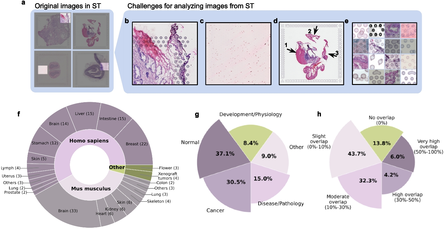
Training data collection

We collected 167 datasets generated by the 10× Visium platform from 49 studies, which were downloaded from STOmics DB [42] and 10× Genomics website [43]. The training images included a total of 21 distinct tissue types, spanning both human and mouse origins as well as various biological conditions (Fig. 1f, g). The full list of studies is provided in Additional file 1: Table S2. To generate training annotations for fiducial marker areas, we applied the Hough circle transform algorithm [44], which uses pixel intensity to identify circular shapes in images. However, the algorithm produced numerous false positives in tissue regions and missed certain markers due to deformations or overlap with tissue areas. To address these limitations, we manually removed false positives and annotated markers missed by the Hough circle transform using the Labelme data annotation tool [45], resulting in a comprehensively annotated dataset containing 92,685 fiducial markers.

Neural network architecture

The neural network employed by Vispro is based on the U-Net architecture [20], a widely recognized neural network design for medical image segmentation. U-Net features a symmetric encoder-decoder structure optimized for efficient feature representation and reconstruction. The encoder progressively extracts hierarchical features through downsampling, while the decoder restores spatial resolution via upsampling, enabling the integration of fine-grained details with contextual information. This fully convolutional architecture ensures seamless feature extraction and reconstruction, making it well-suited for segmentation tasks.

The implementation of Vispro incorporates four UNetDown blocks, each designed to progressively reduce spatial resolution by half while increasing the number of feature channels from the initial 3 (RGB) to 32, 64, 128, and 256, respectively. Each block uses a \(4\times 4\) convolution with a stride of 2, followed by instance normalization and ReLU activation [46], forming the core structure of the UNetDown block.

To address the specific challenges of fiducial marker segmentation, characterized by small-scale structures that are globally distributed but constrained to a square shape, we introduced targeted modifications to the network design. These adjustments prioritize retaining fine-grained details in the initial encoding layers while enhancing global shape awareness in the deepest encoding layers. The network structure is detailed below:

The input of the network is a 3-channel image, i.e., \(I \in \mathbb ^\).

For the first encoding block, additional convolutional layers are added while avoiding dropout to preserve detailed feature extraction.

$$\begin \text ~~~ & \dot^1 = \text _ \left( \text _(I) \right) , \nonumber \\ \text ~~~ & \ddot^1 = \text (\dot^1). \end$$

(1)

For the second and third encoding blocks (\(i=2,3\)), a foundation module is utilized.

$$\begin \text ~~~ & \dot^ = \text _(\ddot^), \nonumber \\ \text ~~~ & \ddot^ = \text (\dot^). \end$$

(2)

For the fourth encoding block, additional convolutional layers are added to enhance feature extraction.

$$\begin \text ~~~ & \dot^4 = \text _ \left( \text _(\ddot^3) \right) , \nonumber \\ \text ~~~ & \ddot^4 = \text (\dot^4). \end$$

(3)

At the end of the encoding operations, additional bottleneck layers are incorporated at the deepest level of the network to further refine the receptive fields of the encoded features, as detailed below:

$$\begin \text ~~~\dot = \text _ \left( \text _(\ddot^4) \right) . \end$$

(4)

To reconstruct spatial context for fine-grained segmentation, the decoder progressively upsamples the bottleneck features through a series of four UNetUp blocks, mirroring the hierarchical structure of the encoder. At each scale, a \(4 \times 4\) deconvolution operation is applied to double the spatial resolution of the learned features while sequentially reducing the feature channels from 256 to 128, 64, 32, and 16. These operations are followed by activation functions and skip connections, which seamlessly integrate high-resolution features from the encoder. This approach ensures the preservation of spatial details and enriches the reconstruction process with complementary contextual information.

Formally, the operations at the first decoding block are defined as follows, with additional convolutional layers applied to both the decoding features and the skip features to enhance global attention:

$$\begin \text ~ & \dot^1 = \text _\left( \text _(\dot)\right) , \nonumber \\ \text ~ & \ddot^1 = \text (\dot^1), \nonumber \\ \text ~ & \ddddot^1 = \ddot^1 + \text _(\ddot^3). \end$$

(5)

For the second decoding block:

$$\begin \text ~ & \dot^2 = \text _(\ddddot^1), \nonumber \\ \text ~ & \ddot^2 = \text (\dot^2), \nonumber \\ \text ~ & \dddot^2 = \ddot^2 + \ddot^2. \end$$

(6)

For the third decoding block:

$$\begin \text ~ & \dot^3 = \text _(\dddot^2), \nonumber \\ \text ~ & \ddot^3 = \text (\dot^3), \nonumber \\ \text ~ & \dddot^3 = \ddot^3 + \ddot^1. \end$$

(7)

For the fourth decoding block:

$$\begin \text ~ & \dot^4 = \text _\left( \text _(\dddot^3)\right) , \nonumber \\ \text ~ & \ddot^4 = \text (\dot^4), \nonumber \\ \text ~ & \dddot^4 = \ddot^4 + I. \end$$

(8)

Each decoder layer processes the learned feature maps \(\dot^i\) while incorporating feature maps \(\dot^i\) from the corresponding encoder layers via skip connections. These skip connections retain spatial details that are otherwise lost during downsampling, enabling the network to effectively merge high-resolution spatial features with deeper contextual information. This synergy significantly enhances the network’s capacity to reconstruct fine-grained features with precision, a critical advantage for segmentation tasks. The Vispro architecture further ensures that the network adeptly captures both intricate details and global context, making it particularly well-suited for segmenting small fiducial markers while maintaining their global shape constraints.

Neural network output

The output of the decoder is a 19-channel feature map at full resolution, comprising 16 learned feature channels and 3 channels from the original input image, i.e., \(\dddot^4 \in \mathbb ^\). This feature map is passed through a learnable final layer, which generates the marker segmentation mask \(\hat\):

$$\begin \hat = \text \left( \text _(\dddot^4)\right) \in [0, 1]^ \end$$

(9)

Loss function

We employed a combined loss function, consisting of Dice Loss [47] and Focal Loss [48], to evaluate the predicted marker mask, \(\hat\), against the gold standard mask, M, obtained through manual annotation. The gold standard mask, M, is a binary mask where 1 represents the fiducial marker region and 0 represents the background region. In contrast, \(\hat\) contains values in the range (0, 1), where values closer to 1 indicate a high likelihood of the marker region, and values closer 0 indicate a high likelihood of the background region.

The Dice Loss, widely used in segmentation tasks, evaluates the overlap between the target regions in the two masks. To calculate the Dice Loss, the predicted mask, \(\hat\), is first binarized by applying a threshold of 0.5, resulting in a binary prediction mask, \(\hat_b\). The Dice Loss is then computed as follows:

$$\begin \text \quad L_d = 1 - \frac_b \cap M| + \epsilon }_b| + |M| + \epsilon } \end$$

(10)

where \(\epsilon\) is a smoothing factor set to \(\epsilon = 1.0\) to stabilize the loss value, especially for small or empty masks.

For the Focal Loss, it builds upon the pixel-wise Binary Cross-Entropy (BCE) Loss and introduces additional parameters to emphasize hard-to-classify markers while down-weighting easy-to-classify markers by adjusting the loss contribution of each example. Specifically, the BCE Loss is defined as:

$$\begin \text \quad L_} = - \frac \sum \limits _^ \left[ y_i \cdot \log (\hat_i) + (1 - y_i) \cdot \log (1 - \hat_i) \right] , \quad y_i \in M, \, \hat_i \in \hat \end$$

(11)

where \(N\) is the total number of pixels, \(y_i\) represents the ground truth label for pixel \(i\), and \(\hat_i\) is the corresponding predicted value from the neural network.

Focal Loss introduces weighting terms that dynamically adjust the loss contributions based on the predicted values of the network. This adjustment is achieved through the following formulation:

$$\begin \text \quad L_f = - \frac \sum \limits _^ \left[ \alpha \cdot y_i \cdot (1 - \hat_i)^\gamma \cdot \log (\hat_i) + (1 - \alpha ) \cdot (1 - y_i) \cdot \hat_i^\gamma \cdot \log (1 - \hat_i) \right] \end$$

(12)

where \(\gamma\) controls the level of focus on hard examples, and \(\alpha\) is a class-level weighting factor used to prioritize the target class. In Vispro, we set \(\alpha = 0.95\) and \(\gamma = 3\).

By inversely scaling the weights based on the confidence levels of predictions, the loss function reduces the impact of well-classified samples while emphasizing harder and misclassified examples. This adaptive weighting mechanism ensures that the network prioritizes challenging samples during training, effectively balancing the contributions of both easy and hard examples to the overall loss.

The total loss used to train the network combines the Dice Loss and Focal Loss, defined as follows:

$$\begin \text \quad L_} =\lambda \cdot L_d + (1 - \lambda ) \cdot L_f \end$$

(13)

where \(\lambda\) is a weighting parameter that balances the contributions of the two loss components, set to \(\lambda = 0.9\) in Vispro.

Training procedure

Since markers located in the background region are more numerous and easier to classify, whereas markers overlapping with tissue regions are fewer and harder to distinguish, we implemented a sampling layer to increase the frequency of challenging samples during network training. Specifically, we computed a slice-wide marker overlap factor, defined as the ratio of in-tissue markers to the total number of markers. Based on this factor, we categorized images into three difficulty levels: hard examples (marker factor > 0.8), moderate examples (0.3 < marker factor \(\le\) 0.8), and easy examples (marker factor < 0.3). To ensure the model effectively learns from the most challenging cases, we increased the occurrence of hard samples threefold and moderate samples twofold in the training dataset.

During training, all images underwent carefully designed data augmentation strategies to enhance data variability and improve model robustness. These augmentations included random flipping (both left-right and up-down), scaling (0.8 to 1.0 times the original size), rotation (\(-10^\circ \text +10^\circ\)), brightness adjustment (0.5 to 1.2 times the original value), and Gaussian blurring (with a standard deviation randomly selected between 0 and 1). The model is trained using the Adam optimizer [49] with a learning rate of \(10^\). The optimizer’s parameters include \(\beta _1 = 0.5\) and \(\beta _2 = 0.999\), which control the exponential decay rates of the first- and second-order moment estimates of the gradients, respectively. These settings ensure stable convergence during training. The network was trained for 800 epochs.

Vispro module 2: image restoration

The second step in Vispro involves performing image restoration on the marker-covered regions of the images. For this task, we leverage LaMa, a deep learning model specifically designed for image inpainting [50]. Image inpainting is a computer vision technique that aims to fill in missing or corrupted regions of an image. The fundamental principle involves learning the surrounding textures and global image semantics to generate visually plausible content for the missing regions.

In this module, we incorporate the pre-trained model and parameters of LaMa [51], which employs Fourier Convolutions [52] to address the limitations of conventional inpainting methods that often struggle to generalize across varying resolutions. This approach ensures consistent performance on both low- and high-resolution images, enabling pre-training on large-scale natural image datasets while seamlessly adapting to ST images, which are typically high resolution.

The input to the model consists of the original image I and the predicted binary mask \(\hat\) generated by Vispro Module 1. The output is an RGB image \(\hat\), where the fiducial marker regions are filled with plausible textures inferred from the surrounding image content.

Vispro module 3: tissue detection

For the task of tissue detection, we employed the deep learning tool backgroundremover [53], which is based on the U²-Net model [21], a state-of-the-art salient object detection framework. The incorporation of Residual U-blocks (RSU) [21] enhances the network’s capacity for efficient hierarchical feature learning, ensuring precise representation of fine-grained details alongside broader spatial patterns, making it particularly adept at robust tissue segmentation, especially in high-resolution images where traditional models frequently struggle to achieve a balance between detail preservation and global contextual accuracy.

By default, Vispro uses the unet2 model and resizes images to 320 \(\times\) 320 to optimize computational efficiency. For datasets with small tissue regions (less than 100 \(\times\) 100 pixels), Vispro increases the image size to 1000 \(\times\) 1000 and switches to the u2netp model. This adjustment enhances detection accuracy for finer structures and thinner tissue regions.

The input to the model is the restored RGB image \(\hat\) produced by Vispro Module 2, and the outputs are a tissue mask \(\hat_t\) with values in the range [0, 1] and a blended RGBA image \(\hat_t\) that visually highlights the detected tissue regions.

Vispro module 4: disconnected tissue segregation

We identified disconnected components in the tissue probability mask \(\hat_t\) using the OpenCV library. Specifically, the probability mask was binarized using a tissue threshold value (default set to 0.8). The label function was then employed to count and label the disconnected regions in the binary mask. This function performs a brute-force search to determine pixel connectivity, iterating through each pixel in the mask and checking for 8-connectivity (including horizontal, vertical, and diagonal neighbors) to ascertain whether adjacent pixels belong to the same component. Once a connected group of pixels is identified, the algorithm assigns a unique integer label to the corresponding component. The output is a labeled mask in which each connected component is represented by a distinct integer value.

The input to this module is the tissue probability mask \(\hat_t\) produced by Vispro Module 3, and the output is a refined segmentation mask \(\hat_s\), represented with integer values.

To improve the quality of the labeled mask, an additional step was introduced to remove small components, often artifacts caused by staining errors or computational inaccuracies near the tissue boundary. These small components were filtered out using a preset area threshold (default set to 20). Any component with an area below this threshold was excluded from the labeled mask. This refinement step ensures that the labeled mask more accurately represents tissue regions and minimizes noise.

Competing methods10× standard processing pipeline

In the 10× pipeline, fiducial markers are processed using Space Ranger [15] and Loupe Browser [16], which generate a layered image. This image includes a fiducial frame template with red circles overlaid on the original H&E image to highlight fiducial marker areas. These tools can automatically detect and highlight the fiducial regions, providing a visual reference for their locations on the tissue. However, they usually require complex model inputs, including gene count data, slide version information, and images. Additionally, in cases where fiducial markers are obstructed or tissue boundaries are unclear, manual alignment is often necessary.

To integrate 10×’s aligenment result into our workflow for evaluation, we first perform an RGB thresholding operation on the layered image to isolate the red color component representing the fiducial markers. This step extracts the red circles by identifying pixels that fall within a predefined range of RGB color intensities (R >180, G<30, and B<30). Once the red components are isolated, we apply a circle detection of Hough circle transform to detect the circular fiducial markers. This algorithm scans the image for circular shapes by identifying edge pixels and fitting circles to the detected contours. After detecting the circles, we fill in each circle area to create a binary mask. In this mask, pixel values are set to 1 within the fiducial marker regions and 0 elsewhere, mimicking the format used in our pipeline. This binary mask is then used for further evaluation, enabling a direct comparison of the performance between the 10× pipeline and Vispro.

Hough circle transform

The Hough circle transform [44] is a classical technique for detecting circular patterns in images by mapping edge-detected points into a parameter space. It identifies curves through a voting process in a discretized accumulator space, making it well suited for detecting parametric shapes such as circles. We adopted the OpenCV implementation with default settings to detect circular features like fiducial markers. This method serves as a non-learning-based baseline in our comparative evaluation.

Cellpose

Cellpose [23] is a generalist algorithm for cell segmentation that performs well across a broad range of cell types and imaging modalities. It models spatial gradients (vector flows) from cell interiors to boundaries to guide mask generation, enabling generalizable performance across domains. We used the pre-trained Cellpose model with the diameter parameter fixed at 25, which corresponds closely to the average fiducial marker size in our dataset. This standard configuration ensures a consistent and fair evaluation.

CircleNet

CircleNet [24] is a deep learning-based framework specifically designed for circle detection, leveraging the hourglass network architecture to capture multi-scale spatial features. The model predicts circle centers and radii directly from the image using convolutional outputs. In our study, we used the hourglass architecture with the pre-trained model provided from the MoNuSeg dataset. This setup enables robust detection of circular structures and serves as a learning-based benchmark.

Baseline U-Net

For the baseline U-Net, we follow the design of pix2pix [46], a widely used U-Net variant for image processing tasks. We adopt its U-Net generator as the baseline for marker segmentation and compare its results with the tailored architecture in Vispro. The network generates fiducial marker masks similar to Vispro, enabling a direct comparison of performance.

Deep image prior

Deep Image Prior [26] (DIP) leverages the structure of a convolutional neural network to perform image restoration without requiring any pre-training. The method is based on the insight that the network architecture itself captures natural image statistics, enabling it to denoise or inpaint images without external datasets. We followed the recommended protocol and trained DIP for 2000 iterations per image to inpaint corrupted or missing regions. This approach serves as an unsupervised benchmark for restoration performance.

Stable diffusion model

Stable Diffusion [27] is a generative model capable of high-fidelity semantic inpainting. It operates by learning a latent representation of images through denoising score matching and iteratively generating plausible content conditioned on a text prompt. We employed the inpainting-specific model runwayml/stable-diffusion-inpainting with the prompt “Fill the masked region seamlessly.” This approach enables content-aware filling of masked tissue regions and serves as a generative baseline.

Otsu

Otsu [17] is a widely used histogram-based thresholding algorithm for binarizing grayscale images. It determines the optimal threshold by maximizing the inter-class variance between foreground and background pixels, making it effective for images with bimodal histograms. We applied OpenCV’s implementation to provide a fast, unsupervised baseline for separating tissue from background.

SAM

The Segment Anything Model [18] (SAM) is a prompt-driven segmentation framework based on vision transformers. It generates segmentation masks by attending to user-provided prompts, such as points or bounding boxes, using a pre-trained image encoder to generalize across diverse object types. We evaluated SAM in two settings: tissue segmentation and tissue segregation. For tissue segmentation, a binary task, we used the image center as a point prompt to extract a confident primary region, which was treated as the tissue area. For tissue segregation, a multi-class segmentation task, we applied the model’s default “segment anything” mode across the entire image. Both settings used the sam_vit_h_4b8939.pth model.

TESLA

Although TESLA [54] was originally developed for gene expression imputation in spatial transcriptomics, it includes a built-in tissue detection module that combines image-derived and transcriptome-derived strategies for boundary estimation. This module incorporates three techniques: (1) Canny edge detection via OpenCV, (2) horizontal projection of transcript spot density along the x-axis, and (3) vertical projection along the y-axis. We applied all three techniques using the default settings.

EvaluationsFiducial marker identification

To evaluate the accuracy of fiducial marker segmentation, we computed the pixel-level Intersection over Union (IoU) using the manually annotated gold standard as a reference. The IoU is a metric that measures the overlap between the predicted mask and the ground truth mask at the pixel level. It is defined as the ratio of the number of correctly predicted pixels (i.e., the intersection of the predicted and ground truth masks) to the total number of pixels in the union of the predicted and ground truth masks:

$$\begin \text = \frac \left( P_ \wedge G_ \right) } \left( P_ \vee G_ \right) } \end$$

(14)

where \(P_\) represents the predicted mask at pixel location \((i, j)\), \(G_\) represents the ground truth mask at pixel location \((i, j)\), \(\wedge\) denotes the logical AND operation (i.e., the number of pixels where both \(P_ = 1\) and \(G_ = 1\), representing the intersection), and \(\vee\) denotes the logical OR operation (i.e., the number of pixels where either \(P_ = 1\) or \(G_ = 1\), representing the union). A higher IoU value indicates a higher segmentation accuracy, as it shows that the predicted mask aligns more closely with the ground truth mask.

All images were divided into 12 groups for 12-fold cross-validation. In each iteration, images from 11 groups were used for training, while images from the remaining group were used for testing.

Identifying tissue regions

To assess the accuracy of tissue region segmentation, we manually annotated tissue regions on 21 tissue slices (Additional file 1: Table S3), encompassing a spectrum of difficulty from straightforward to challenging cases.

To quantitatively assess segmentation performance, we employed three metrics that capture both regional accuracy and boundary shape characteristics: Intersection over Union (IoU), Hausdorff Distance (HD), and Perimeter Ratio (PerimRatio).

IoU measures the overlap between the predicted mask P and the ground truth mask G, defined as:

$$\begin \textrm(P, G) = \frac. \end$$

(15)

The average IoU is computed by taking the mean of \(\textrm(P_i, G_i)\) over all samples.

Hausdorff Distance measures the maximum distance between points on the predicted boundary \(\partial P\) and the closest points on the ground truth boundary \(\partial G\):

$$\begin \textrm(P, G) = \max \left\ \inf _ d(p, g),\ \sup _ \inf _ d(g, p) \right\} , \end$$

(16)

where \(d(\cdot ,\cdot )\) is the Euclidean distance. The average HD is obtained across all samples.

To assess boundary complexity relative to the ground truth, the perimeter ratio is defined as:

$$\begin \textrm(P, G) = \frac. \end$$

(17)

This ratio identifies cases of over- or under-segmentation with excessive or insufficient boundary delineation.

Segregating disconnected tissue regions

To evaluate the accuracy of tissue segregation, we computed both the IoU and the difference in the number of connected components between the predicted mask P and the ground truth G. The IoU is defined above. The difference in the number of components is calculated as:

$$\begin \textrm(P, G) = \left| N(P) - N(G) \right| , \end$$

(18)

where \(N(\cdot )\) denotes the number of connected components in a binary mask. This metric captures both over-segmentation (excess components) and under-segmentation (merged regions), providing a measure of the topological fidelity of the prediction.

Cell segmentation

To evaluate cell segmentation performance, we utilized StarDist [30, 55, 56] to detect cells in both the original H&E images and the images processed by Vispro. Evaluation was performed on 20 tissue slices with microscopy-resolution images (Additional file 1: Table S3). StarDist is a state-of-the-art segmentation algorithm designed for star-convex object detection in both 2D and 3D images, making it particularly well-suited for accurately segmenting objects with varying shapes and sizes, such as nuclei in histopathological images. We employed the 2D_versatile_he model, pre-trained for H&E-stained histological images. The main model parameters were configured as follows: block_size was set to 4096, prob_threshold to 0.01, and nms_threshold to 0.001.

To compute the PCA projections of cell morphological features, we extracted the following descriptors: area, perimeter, elongation, eccentricity, circularity, solidity, extent, aspect ratio, and compactness. Each feature was then standardized to have a mean of 0 and a standard deviation of 1 across cells. PCA was applied to the scaled feature set, and the projections onto the first two principal components were visualized.

For cell segmentation results obtained by each method, we calculated the number of segmented cells falling outside of the manually annotated tissue regions.

Image registration

We evaluated the accuracy of image registration in both same-modal and cross-modal settings. For the same-modal setting, we used 20 pairs of Visium images from our collected dataset (Additional file 1: Table S3), where each pair originated from the same study and shared similar textures. For the cross-modal setting, we collected 13 pairs of images from the Visium CytAssist dataset (Additional file 1: Table S4). This dataset involves overlaying images of standard histological glass slides with those processed into Visium slides. While structurally identical, the pairs exhibit slight texture differences, making them ideal for testing cross-modal registration performance.

We included two competing methods for evaluation. The first is bUnwarpJ registration [57], available within the ImageJ/Fiji software [32], for image registration. bUnwarpJ performs 2D image registration using elastic deformations modeled by B-splines, ensuring invertibility through a consistency constraint. We used the stable version (2.6.13) of the software, configuring the initial deformation to coarse, the final deformation to super fine, while leaving all other parameters at their default settings. The second is SimpleITK, a tool for image registration that supports rigid, affine, and deformable transformations with customizable similarity metrics, optimizers, and interpolators. We used version 2.4.0 of the software with default settings.

Three metrics were used for quantitatively evaluations. The first metric is the Structural Similarity Index (SSIM), which measures the similarity between two images by comparing local patterns of pixel intensities, normalized for differences in luminance and contrast. SSIM is particularly sensitive to pixel misalignment, making it a robust metric for evaluating registration performance, especially in the context of same-modal image registration. For the multi-channel data in our case (i.e., RGB with three channels), SSIM is calculated separately for each channel, and the final metric is obtained by averaging the scores across all channels. This approach ensures a comprehensive evaluation of structural similarity for color images. For each channel, the SSIM is mathematically defined as:

$$\begin \text (I_x, I_y) = \frac \sum \limits _^ \frac^k + c_2)} + \mu _y^ + c_1)(\sigma _x^ + \sigma _y^ + c_2)}, \end$$

(19)

where \(I_x\) and \(I_y\) are the two input images, N is the total number of local image patches. \(\mu _x^k\) and \(\mu _y^k\) represent the local means, \(\sigma _x^k\) and \(\sigma _y^k\) are the local standard deviations, and \(\sigma _^k\) denotes the cross-covariance of the intensity values in the kth patch of \(I_x\) and \(I_y\). The constants \(c_1\) and \(c_2\) are stability parameters introduced to prevent division by zero.

The second metric is Mutual Information (MI), which quantifies the amount of information shared between two random variables and is widely used in image registration tasks to measure the similarity between images. As MI is calculated from whole-image pixel patterns, it excels at identifying alignment by leveraging structural and contextual consistency rather than relying on simple intensity correspondence, making it particularly effective for estimating registration tasks involving images from different modalities. To handle the continuous intensity values in the image pair \(I_x\) and \(I_y\), the pixel intensities are first discretized into bins using a 2D histogram. Each bin represents a range of intensity values, and the histogram captures the co-occurrence of intensity values from the two images at corresponding spatial locations. The 2D histogram is then normalized to estimate the joint probability distribution p(x, y), as well as the marginal probabilities p(x) and p(y), where x and y represent the bins of intensity values from \(I_x\) and \(I_y\), respectively. These probabilities are then used to compute MI.

Formally, MI is calculated as follows:

$$\begin \text (I_x, I_y) = \sum \limits _ \sum \limits _ p(x, y) \log \left( \frac \right) , \end$$

(20)

The third metric is the Dice score, which is used to assess the agreement between expert-annotated cortical layers after performing image registration on the DLPFC dataset [35]. The Dice score is a widely used metric for measuring the similarity between two sets and is particularly well-suited for assessing multi-class area overlap in spatial segmentation tasks. Specifically, we extracted the convex hulls of manually annotated cortical layers in both the target and source images after performing image registration with different methods. These convex hulls were converted into image-format masks, where distinct pixel values represented different tissue layers. The Dice score was then computed to quantify the spatial overlap between corresponding layers.

Given two segmentation masks, \(I_x\) and \(I_y\), corresponding to the target image and the source image after registration, respectively. The Dice score is defined as:

$$\begin \textrm(I_x, I_y) = \frac \sum \limits _^ \frac. \end$$

(21)

where \((I_x = c)\) and \((I_y = c)\) denote the sets of pixels assigned to class \(c\) in the target and source images, respectively. This formulation captures both over-segmentation and under-segmentation across tissue regions and reflects the topological fidelity of the registration.

Gene imputation

We employed the TESLA software for gene imputation [54]. TESLA leverages the Canny edge detection algorithm from the OpenCV library for contour detection and also offers alternative methods based on the spatial locations of transcripts. We tested all three contour detection methods provided by TESLA and conducted a detailed visual comparison of the imputation outcomes (Additional file 1: Table S5). For consistency, the imputation resolution was set to 50 during implementation.

After performing gene imputation using TESLA, we further conducted spatial domain detection. Specifically, we utilized the standard Seurat pipeline [58] to perform library size normalization, log transformation, highly variable gene selection, and PCA on the imputed gene expression counts. We then applied k-means clustering to the PCA embeddings to obtain cell cluster labels. The resulting spatial domain labels were then projected back onto the original spot coordinates based on nearest-neighbor matching. Finally, the Adjusted Rand Index (ARI) was used to compare the predicted spatial domains with manual annotations.

The ARI is defined as:

$$\begin \textrm = \frac \left( n_\\ 2\end}\right) - \left[ \sum _i \left( a_i\\ 2\end}\right) \sum _j \left( b_j\\ 2\end}\right) / \left( n\\ 2\end}\right) \right] } \left[ \sum _i \left( a_i\\ 2\end}\right) + \sum _j \left( b_j\\ 2\end}\right) \right] - \left[ \sum _i \left( a_i\\ 2\end}\right) \sum _j \left( b_j\\ 2\end}\right) / \left( n\\ 2\end}\right) \right] }, \end$$

(22)

where \(n_\) is the number of elements shared between predicted cluster \(i\) and true cluster \(j\), \(a_i\), and \(b_j\) are the numbers of elements in predicted cluster \(i\) and true cluster \(j\), respectively, and \(n\) is the total number of elements. The ARI ranges from 0 (random labeling) to 1 (perfect match), providing a robust measure of clustering agreement.