Curating HiChIP and ChIP-seq samples

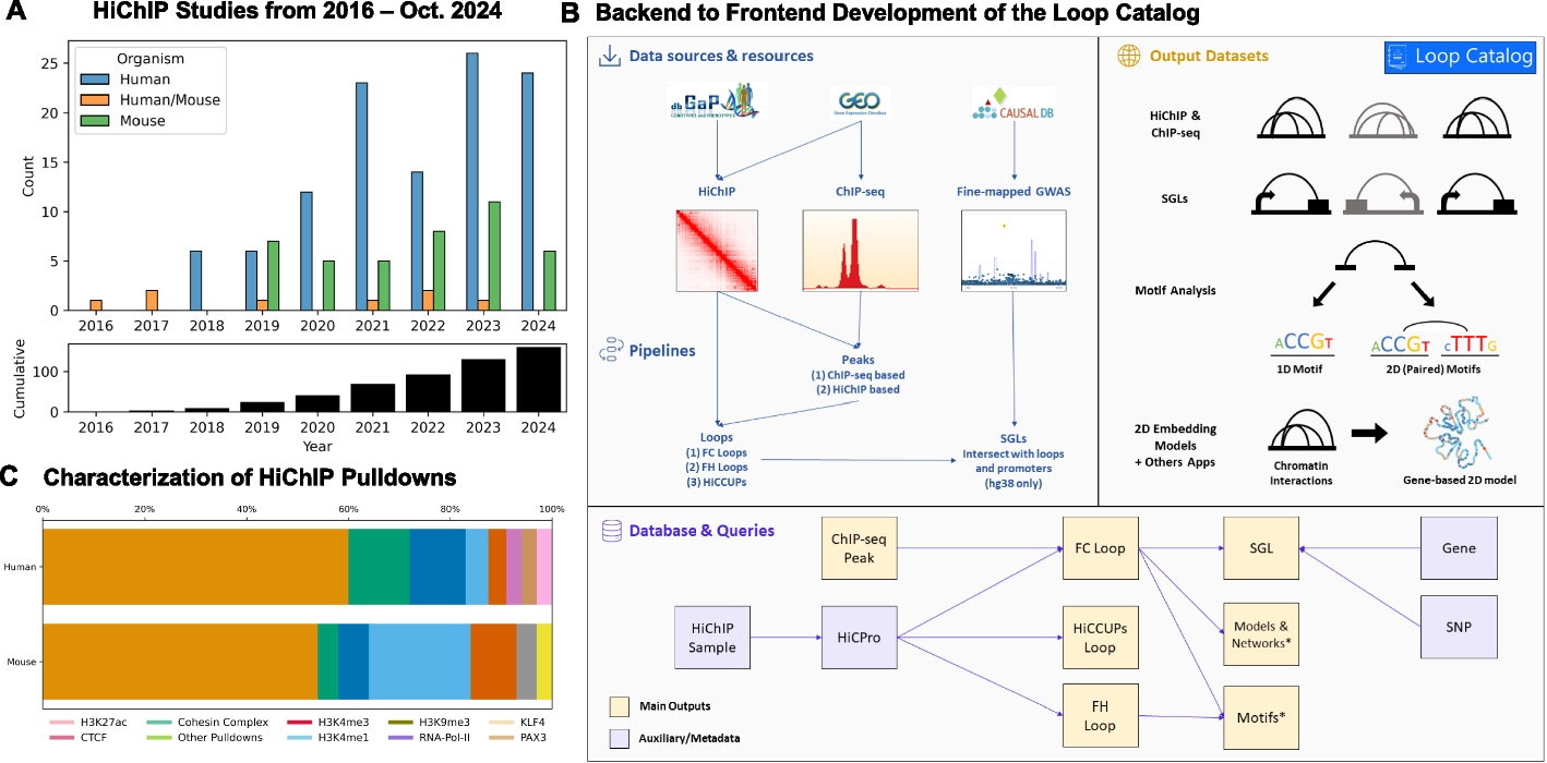
To identify a comprehensive list of publicly released HiChIP datasets, we developed a pipeline that scans NCBI’s Gene Expression Omnibus (GEO) database [52] for studies performing HiChIP experiments. To extract information on these studies, the BioPython.Entrez [53] and metapub.convert (https://pypi.org/project/metapub/) packages were used. Raw sequencing data associated to these studies was then identified from the Sequence Read Archive (SRA) database using the pysradb Python package (https://github.com/saketkc/pysradb), and the results were manually examined to extract HiChIP samples. ChIP-seq samples corresponding to these studies were also extracted if there was a record of them with the same GEO ID as the HiChIP sample.

Populating sample metadata

To automatically add metadata such as organ and cell type to the curated HiChIP data, the BioPython.Entrez package was used to perform a search query within the GEO database. GSM IDs from the previous query were used with an esummary query to the biosample database [53]. From these results, organism, biomaterial, celltype, GSM ID, SRA ID, disease, organ, treatment, tissue, and strain (only for mouse) were extracted. To improve classes for organ and biomaterial, a dictionary of classes as keys and synonyms as value (e.g., heart is a key and its synonyms are cardiovascular, atrium, aorta) was used to search across GEO and Biosample reports. “N/A” was used to indicate fields that were not applicable for a given sample, and, for the remaining fields, “Undetermined” was assigned when the information could not be retrieved.

Downloading raw sequencing datasets

HiChIP FASTQ files were systematically downloaded using one of three methods and prioritized in the following order: SRA-Toolkit’s prefetch and fasterq-dump (2.11.2) (https://hpc.nih.gov/apps/sratoolkit.html), grabseqs (0.7.0) [54], or European Bioinformatics Institute (EBI) URLs generated from SRA Explorer (1.0) [55]. In addition, FASTQ files for phs001703v3p1 and phs001703v4p1 which pertain to two previously published HiChIP studies from the Database of Genotypes and Phenotypes (dbGaP) were downloaded [6, 44, 56] (Additional file 2: Table S1). Additionally, ChIP-seq FASTQ files were downloaded from GEO using grabseqs (0.7.0).

Processing reads from HiChIP data

HiChIP sequencing reads from human samples were aligned to hg38 while reads from mouse samples were aligned to mm10 using the HiC-Pro (3.1.0) pipeline [57] (Additional file 3: Table S2). Reference genomes were downloaded for hg38 (https://hgdownload.soe.ucsc.edu/goldenPath/hg38/bigZips/) and for mm10 (https://hgdownload.soe.ucsc.edu/goldenPath/mm10/bigZips/) and indexed with bowtie2 (2.4.5) [58] using default parameters. Chromosome size files for hg38 and mm10 were additionally retrieved from these repositories. FASTQ files for all technical replicates of a HiChIP biological replicate were processed together by HiC-Pro. Restriction enzymes and ligation sequences were determined during the HiChIP literature search (Additional file 4: Table S3), and restriction fragments were generated with the HiC-Pro digestion.py tool using default parameters. FASTQ files were split into chunks of 50,000,000 reads using the HiC-Pro split_reads.py utility, and HiC-Pro was run in parallel mode with a minimum mapping quality (MAPQ) threshold of 30. Invalid pairs (singleton, multi-mapped, duplicate, etc.) were removed. Raw and ICE (Iterative Correction and Eigenvector Decomposition) normalized contact matrices were generated at the 1 kb, 2 kb, 5 kb, 10 kb, 20 kb, 40 kb, 100 kb, 500 kb, and 1 mb resolutions. For all other HiC-Pro configuration parameters, the defaults were used. Exceptions to this workflow are as follows:

(1)

For MNase HiChIP samples, R1 and R2 FASTQ reads were trimmed from the 3′ end to 50 bp to account for the increased likelihood of chimeric reads. HiC-Pro was run with MIN_CIS_DIST=1000 specified to discard non-informative pairs. Validpairs generated from this HiC-Pro configuration were used for loop calling. HiC-Pro was additionally run for all MNase HiChIP samples without the MIN_CIS_DIST parameter specified to enable the collection of short valid pairs which are required by the FitHiChIP PeakInferHiChIP.sh utility (10.0) [59] to infer peaks from HiChIP. Valid pairs generated from this HiC-Pro configuration were used only for peak inference from HiChIP data.

(2)

For Arima HiChIP samples derived from studies conducted in late 2022 or later and with an R1 or R2 mapping percentage less than 80% reported by our default HiC-Pro configuration, 5 bp were trimmed from the 5′ end of the R1 and R2 FASTQ reads to remove the Arima adaptor sequence. HiC-Pro was then re-run as initially specified.

Juicer (2.0; juicer_tools.jar 2.20.00) [60] was applied to a subset of HiChIP samples. Reference genomes for hg38 and mm10 were obtained as previously described and indexed using BWA index (0.7.17) [61] with default parameters. Restriction enzymes were determined as previously described, and restriction sites were generated using the Juicer generate_site_positions.py utility. HiChIP technical replicates were combined and processed together. juicer.sh was run with the appropriate indexed reference genome, chromosome sizes file, restriction enzyme, and restriction sites. HiChIP FASTQs were split into chunks of 50,000,000 reads (-C 50000000) and the --assembly flag as formatted in earlier versions of HiCPro merged_nodups pairs file. For MNase HiChIP samples, the restriction enzyme was set to “none” (-s none) and no restriction site file was provided. Pairs were filtered according to a minimum MAPQ threshold of 30. Statistics reported in the inter_30.txt file were extracted for alignment tool comparison analyses.

The distiller-nf pipeline (0.3.4) [62] was run using Nextflow (22.10.7) [63] for a subset of HiChIP samples. HiChIP technical replicates were combined and processed together. distiller-nf was run with the appropriate reference genome and chromosome sizes file. Mapping was performed with a chunk size of 50,000,000 reads and with the use_custom_split option set to “true.” Read alignments were parsed with options --add-columns mapq and --walks-policy mask. Duplicates were detected with max_mismatch_bp set to 1. Pairs with the UU (unique-unique) or UR/RU (unique-rescued) classification and with a MAPQ of at least 30 were retained and used for downstream analyses.

Processing reads and calling peaks for ChIP-seq data

We utilized our previously developed ChIPLine pipeline (https://github.com/ay-lab/ChIPLine) for ChIP-seq processing (Additional file 5: Table S4). ChIP-seq reads were aligned to hg38 for human samples or to mm10 for mouse samples with bowtie2 (2.4.5) with the -k 4 and -X 2000 options specified and defaults otherwise. Uniquely mapped reads were determined using samtools (1.9) [64] to remove random and mitochondrial reads and to impose a minimum MAPQ threshold of 30. PCR duplicates were marked and removed using Picard Tools (2.7.1) [65] with a validation stringency of LENIENT. Several data quality metrics were computed through cross-correlation analysis using the run_spp.R utility from phantompeakqualtools (1.14) [66, 67]. Alignment files were converted into bigwig format for visualization using (1) the UCSC fetchChromSizes, genomeCoverageBed, bedSort, and bedGraphToBigWig utilities [68] for generation of unnormalized bigwigs and (2) deepTools bamCoverage (3.5.1) [69] with -of bigwig, -bs 10, --normalizeUsing RPKM, and -e 200 options specified for generation of bigwigs normalized with respect to coverage. Narrow peaks were derived using MACS2 (2.2.7.1) [70] (Additional file 6: Table S5) with the --nomodel, --nolambda, --shift 0, --extsize 200, and -p 1e-3 parameters specified. For ChIPMentation data, a shifted tagAlign file for peak calling was first constructed by shifting the forward strand by 4bp and reverse strand by 5bp to cover the length of the transposon, and the --bw 200 parameter was additionally specified for MACS2. If available, the corresponding input ChIP-seq files were used by MACS2 for peak calling using the input vs. treatment mode. MACS2 peak calls were made without an input file if no such file was available for the sample. For ChIP-seq datasets with multiple biological replicates, the sequence files for all replicates were processed together to obtain the set of pooled ChIP-seq peaks. Narrow peaks were filtered using a q-value threshold of 0.01 before use in all downstream analyses.

Calling peaks from reads of HiChIP data

In the absence of corresponding ChIP-seq data for a given HiChIP sample from the same study, we inferred peaks directly from HiChIP. We called HiChIP peaks with the PeakInferHiChIP.sh utility script from FitHiChIP, which requires the reference genome, read length (as reported by SRA Run Selector), and processed interaction pairs generated by HiC-Pro (valid, religation, self-circle, and dangling-end pairs) as input and utilizes MACS2 for peak calling (Additional file 6: Table S5). If read lengths differed across technical replicates for a single HiChIP biological replicate, the mode read length was used. For cases in which there was no single mode read length, the longest read length was selected. For merged biological replicates, the mode read length of all individual biological replicates for a given sample was chosen, and similarly, the longest read length was selected in the case of multiple modes.

For comparison purposes, for a subset of HiChIP samples, HiChIP-Peaks peak_call (0.1.2) [71] was run using the correct chromosome size file and HiC-Pro interaction pairs. Restriction fragments were generated with the HiC-Pro digestion.py tool using default parameters. We used a false discovery rate (FDR) of 0.01 (-f 0.01) for peak calling with HiChIP-Peaks.

Performing recall analysis of 1D peaks inferred from HiChIP data

Peaks called from ChIP-seq datasets were considered the ground truth peak set. Peaks inferred directly from HiChIP datasets were assessed for their overlap with ChIP-seq peaks (Additional file 1: Fig. S2), and we computed the percentage of ChIP-seq peaks recovered using HiChIP-inferred peaks. HiChIP and ChIP-seq peak sets were intersected using bedtools intersect (2.30.0) [72] allowing for 1 kb slack on both sides of the peak.

Integration of biological replicates of HiChIP data

In order to generate more deeply sequenced contact maps from the initial set of samples, we combined HiChIP biological replicates from the same study for both human and mouse datasets (Additional file 2: Table S1). Before merging biological replicates, reproducibility was assessed using hicreppy (0.1.0) which generates a stratum-adjusted correlation coefficient (SCC) as a measure of similarity for a pair of contact maps (https://github.com/cmdoret/hicreppy) (Additional file 7: Table S6). Briefly, contact maps in hic format were converted to cool format for hicreppy input at 1 kb, 5 kb, 10 kb, 25 kb, 50 kb, 100 kb, 250 kb, 500 kb, and 1 mb resolutions using hic2cool (0.8.3) (https://github.com/4dn-dcic/hic2cool). hicreppy was run on all pairwise combinations of biological replicates from a given HiChIP experiment. First, hicreppy htrain was used to determine the optimal smoothing parameter value h for a pair of input HiChIP contact matrices at 5 kb resolution. htrain was run on a subset of chromosomes (chr1, chr10, chr17, and chr19) and with a maximum possible h-value of 25. Default settings were used otherwise. Next, hicreppy scc was run to generate a SCC for the matrix pair using the optimal h reported by htrain and at 5 kb resolution considering chr1, chr10, chr17, and chr19 only. A group of HiChIP biological replicates were merged if all pairwise combinations of replicates in that group possessed a SCC greater than 0.8 (Additional file 1: Fig. S3). We merged biological replicates by concatenating HiC-Pro valid pair files before performing downstream processing.

Identifying significant chromatin loops from HiChIP data

Loop calling was performed for both unmerged and merged HiChIP biological replicates by (a) HiCCUPS (JuicerTools 1.22.01) [19, 60], (b) FitHiChIP with HiChIP-inferred peaks (FH loops), and (c) FitHiChIP with ChIP-seq peaks (FC loops), when available [59] (Additional file 8: Table S7). Briefly, HiC-Pro valid pair files for each sample were converted to .hic format using HiC-Pro’s hicpro2juicebox utility with default parameters. HiCCUPS loop calling was initially performed for chr1 only using vanilla coverage (VC) normalization with the following parameters: --cpu, --ignore-sparsity, -c chr1, -r 5000,10000,25000, and -k VC. Samples which passed the thresholds of at least 200 loops from chromosome 1 for human samples and at least 100 loops from chromosome 1 for mouse samples, both at 10 kb resolution, were processed further with HiCCUPS for genome-wide loop calling using the same parameters. For comparison purposes, for a subset of samples, HiCCUPS loop calling was performed with alternative normalization approaches: KR (Knight Ruiz), VC_SQRT (square root vanilla coverage), and SCALE by specifying the -k KR, -k VC_SQRT, and -k SCALE parameters respectively. FitHiChIP peak-to-all loop calling was run with HiC-Pro valid pairs as input at the 5 kb, 10 kb, and 25 kb resolutions for both the Stringent (S) and Loose (L) background models and with coverage bias regression, merge filtering, and an FDR threshold of 0.01. The lower distance threshold for interaction between any two loci was 20 kb and the upper distance threshold was 2 mb; interactions spanning a distance outside this range were not considered for statistical significance.

Loop overlap and aggregate peak analysis

For overlap between two sets of loops, we used either no slack (comparison of normalization methods) or a slack of ± 1 bin (alignment pipeline comparison). For aggregate peak analysis (APA), we used the APA function from the GENOVA [73] R package. APA score was computed as the value of the center pixel divided by the mean of pixels 15–30 kb downstream of the upstream loci and 15–30 kb upstream of the downstream loci [74]. APA ratio was computed as the ratio of central bin to the remaining matrix. For the alignment method comparison analysis, APA was performed for all loops and the top 10,000 significant FitHiChIP loops by q-value called using each alignment method (HiC-Pro, Juicer, or distiller-nf) with respect to the ICE-normalized contact matrix from each respective alignment tool. For the HiCCUPS normalization comparison analysis, APA was performed for the top significant HiCCUPS loops by the “donut FDR” for each normalization method (SCALE, VC, VC_SQRT) using the HiC-Pro-generated ICE-normalized contact matrix as background.

Comprehensive quality control (QC) of HiChIP and ChIP-seq samples

To evaluate sample quality and assign QC flags to all HiChIP (unmerged and merged biological replicates) and ChIP-seq samples, we selected and aggregated a comprehensive set of quality metrics from each processing step: read alignment, peak calling, and loop calling. For FH loops, HiChIP pre-processing was evaluated by number of reads, number of valid pairs, mean mapping percentage, and percentages of valid pairs, duplicate pairs, cis pairs, and cis long-range pairs, HiChIP peak calling was evaluated by number of peaks, and loop calling was evaluated by number of loops (Additional file 9: Table S8). For FC loops, HiChIP read alignment, ChIP-seq peak calling, and loop calling were evaluated as previously described (Additional file 9: Table S8). ChIP-seq pre-processing was evaluated by NRF (non-redundant fraction), PBC1 (PCR bottlenecking coefficient 1), PBC2 (PCR bottlenecking coefficient 2), NSC (normalized strand cross-correlation coefficient), and RSC (relative strand cross-correlation coefficient) (Additional file 5: Table S4).

For each individual metric, QC scores were derived as follows. Based on the distribution of a given metric, along with field standards, we established three numerical intervals that are qualitatively considered “Poor,” “Warning,” and “Good” for that metric defined by thresholds \(_\) and \(_\) (Additional file 10: Table S9). For each metric, we assigned samples a score between 0 and 10, with the 0 to 6 score interval representing “Poor,” 6 to 8 corresponding to “Warning,” and 8 to 10 to “Good,” by performing piecewise linear normalization of metric values. Samples were assigned a score of 10 if their metric value reached the maximum value (for bounded metrics) or was an upper outlier (\(exceed\;the\;75th\;percentile+1.5*InterquartileRange\)). Otherwise, the metric value \(\chi_i\) for sample \(i\) was linearly re-scaled using a weight defined by \(\beta\chi_i=\frac}}\), where:

$$\beta\chi_i=\frac\;if\;min\;<=\chi_i$$

$$\beta\chi_i=\fracif\;t_1<=\chi_i$$

$$\beta\chi_i=\fracif\;\chi_i>=t_2$$

The metric score for sample \(i\) was then defined as \(\beta_\ast\chi_i\) . For metrics for which higher values corresponded to poorer quality, such as duplicate pairs, this score was adjusted by calculating the complement \(10-_\) . To aggregate individual metric scores from one processing step, such as read alignment, we calculated an average of the scores:

where \(m\) is the number of metrics used. Samples were assigned a QC flag for each processing stage based on \(_\) as follows:

A final QC flag of “Poor,” “Warning,” or “Good” was derived for each configuration of loop calling (stringent 5 kb, loose 5 kb, stringent 10 kb, loose 10 kb, stringent 25 kb, loose 25 kb based on processing stage-specific QC flags) (Additional file 1: Fig. S4). “Good” was only assigned in cases where all stage-specific QC flags were “Good.” All other possible cases are further described in Additional file 10: Table S9. The final QC flag assigned to the merge filtered loops is equivalent to that of the non-merge filtered loops for the same sample.

QC flags are displayed within the main data table and on individual sample pages for visual inspection. Additionally, QC flags are automatically downloaded from the main data page (via the “CSV” button), even when the corresponding columns are not visible.

Establishing sets of high-confidence HiChIP samples

We established a high-confidence set of 54 unique human H3K27ac HiChIP samples from the pool of 156 human H3K27ac HiChIP datasets (merged or unmerged biological replicates) with either “Good” or “Warning” QC flags and over 10,000 stringent 5 kb FC loops, henceforth called the High-Confidence Regulatory Loops (HCRegLoops-All) sample set. We additionally established two subsets of the HCRegLoops-All sample set as follows: HCRegLoops-Immune contains 27 samples from immune-associated cell types and HCRegLoops-Non-Immune contains 27 samples from non-immune cell types (Additional file 11: Table S10). Additionally, we defined a CTCF HiChIP sample set of 11 unique samples from the pool of 30 CTCF HiChIP datasets (merged or unmerged biological replicates) with either “Good” or “Warning” QC flags and over 2000 stringent 5 kb FC loops which we call the High Confidence Structural Loops (HCStructLoops) sample set (Additional file 11: Table S10).

Identifying significant chromatin loops from high resolution Hi-C data

Loop calling was performed for 44 high-resolution Hi-C samples gathered from the “High-Resolution Hi-C Datasets” Collection of the 4DN Data Portal (https://data.4dnucleome.org) using Mustache (v1.0.1) [75]. Processed .hic files were downloaded and Mustache was run with default parameters across chr1 through chr22 using raw, KR, and VC normalized contact matrices (-norm) to determine loops at 1 kb, and 5 kb resolutions (-r) (Additional file 12: Table S11).

Identifying SGLs in immune-based diseases

SGLs were identified utilizing fine-mapped GWAS SNPs from CAUSALdb for type 1 diabetes (T1D), rheumatoid arthritis (RA), psoriasis (PS), and atopic dermatitis (AD) which included 7, 7, 3, and 1 individual studies, respectively (Additional file 13: Table S12). The fine-mapped data was downloaded and lifted over from hg19 to hg38 using the MyVariantInfo Python package (version 1.0.0) [76]. We downloaded the GENCODE v30 transcriptome reference, filtered transcripts for type equal to “gene,” and located coordinates of the transcription start site (TSS) [77]. For genes on the plus strand, the TSS would be assigned as a 1-bp region at the start site and, for the minus strand, the 1-bp region at the end site. Lastly, we extracted all HiChIP samples whose organ was classified as “Immune-associated.” To integrate these datasets, loop anchors were intersected with fine-mapped GWAS SNPs and TSSs independently using bedtools pairtobed. Subsequently, loops were extracted as an SGL if at least one anchor contained a GWAS SNP and the opposing anchor contained a TSS.

Calculating significance for the number of SGL links

To assess the number of links we find through SGL mapping in comparison to linking all nearby genes, we built a null distribution. We downloaded all associations from the GWAS Catalog (1.0) (https://www.ebi.ac.uk/gwas/docs/file-downloads), filtered for variants with a p-value less that 5e−8 and linked each SNP to gene within 1 Mb in either direction. A null distribution for the number of SNPs linked to genes, or vice versa, was calculated. We then used a left-sided Mann-Whitney test (scipy.stats.mannwhitneyu with alternative='less') to assign the probability that the number of linked SNPs or genes was less (i.e., more specific) for the SGL approach compared to the null distribution.

Identifying SGLs with immune-associated eQTL studies

SGLs were identified utilizing eQTLs from the eQTL Catalog which included CD4+ T cells, CD8+ T cells, B cells, natural killer (NK) cells, and monocytes (Additional file 14: Table S13). Similarly to GWAS-SGLs, we used GENCODE v30 to locate the TSS and extracted a subset of the GWAS-SGL HiChIP samples whose cell type matched the eQTL studies. To integrate these datasets, loops were intersected with pairs of SNP-gene pairs using bedtools pairtopair. Subsequently, loops were extracted as an SGL if at least one anchor contained an eQTL SNP and the opposing anchor contained a promoter.

Building a consensus gene list for T1D

From the MalaCards database (https://www.malacards.org/), a query was made using the term “type_1_diabetes_mellitus” and the list of associated genes was downloaded. For eDGAR (https://edgar.biocomp.unibo.it/gene_disease_db/), “diabetes mellitus, 1” was queried under the Main Tables tab and all gene symbols were extracted. OpenTargets hosts a disease-based search with gene association scores and a query was made to the MONDO ID for T1D (MONDO_0005147). The corresponding genes were downloaded and filtered for an association score > 0.5. For the GWAS Catalog, a query was made using the previous MONDO ID and all associated genes were extracted. Table 1 of Klak et al. [78] summarizes genes that have been associated with T1D and gene symbols were extracted from this resource.

Performing motif enrichment analysis across conserved anchors

Motif enrichment analysis was performed on conserved loop anchors from the HCRegLoops-All, HCRegLoops-Immune, HCRegLoops-Non-Immune, and HCStructLoops sample sets respectively. Briefly, for each sample set, we identified highly conserved loop anchors by aggregating the merge-filtered 5-kb FC Loops across all samples in the set, extracting unique anchors, and selecting anchors involved in at least one loop call in at least approximately 80% of samples from the sample set (44/54 samples for HCRegLoops-All, 22/27 samples for HCRegLoops-Immune and HCRegLoops-Non-Immune, and 9/11 for HCStructLoops). Conversion from BED to FASTA was performed using the MEME bed2fasta utility (5.5.0). Repeats were masked using TRF (4.10.0) [79] with a match weight of 2, mismatch penalty of 7, indel penalty of 7, match probability of 80, indel probability of 10, minscore of 50, and maxperiod of 500 with the options -f -h -m specified. A biologically relevant background set of sequences was designed by first aggregating all non-conserved loop anchors, converting from BED to FASTA, and performing repeat masking. The non-conserved anchors were then downsampled to the number of conserved anchors using stratified sampling to match the GC content of the foreground conserved anchors. In short, non-conserved anchors were assigned to 0.5% quantiles based on GC content, and for each conserved sequence, GC content was computed and a non-conserved anchor from the corresponding quantile was sampled. We downloaded 727 known human motifs from the 2022 JASPAR CORE database [80]. Motif enrichment analysis was directly applied to the conserved anchor sites using the downsampled non-conserved anchor sites as background using MEME Suite Simple Enrichment Analysis (SEA) (5.5.0) [51] with a match e-value threshold of 10 (Additional file 15: Table S14).

Identifying pairs of motifs overlapping loop anchors

Briefly, for each sample in HCRegLoops-All and HCStructLoops, unique merge-filtered 5-kb FC loop anchors were extracted and these were intersected with sample-specific corresponding ChIP-seq peaks using bedtools intersect with no slack. We selected the peak with the highest signal value to represent that anchor for cases in which multiple H3K27ac peaks overlapped one loop anchor. The resulting peak sets were deduplicated since a single peak may overlap multiple loop anchors. To determine the genomic coordinates of motifs from the 2022 JASPAR CORE database (n = 727 motifs) in these representative peak sets, MEME Suite Find Individual Motif Occurrences (FIMO) (5.5.0) [81] was applied to the HCRegLoops-All sample set on a sample-by-sample basis using a match q-value threshold of 0.01 and default values for all other parameters. For each sample, we intersected motif coordinates with loop coordinates using bedtools pairtobed and annotated loop anchors with the motifs falling within the anchor.

Performing enrichment analysis for motif pairs

Statistical analyses were performed via a bootstrapping method for HCRegLoops-All HiChIP samples (Additional file 16: Table S15, Additional file 1: Fig. S5). To avoid shuffling with unmappable or repeat regions, we excluded loops where either anchor overlapped blacklisted regions from https://github.com/Boyle-Lab/Blacklist/blob/master/lists/hg38-blacklist.v2.bed.gz. We designed a block bootstrap approach with anchors as the unit analysis and anchors were randomly shuffled within their corresponding chromosomes. To then build a null distribution, we performed 100,000 simulations where we assigned a uniform probability of drawing a given anchor within each chromosome with replacement. P-values were determined for each sample by counting the total number of simulated pairs greater than or equal to observed pairs in the original sample. Due to the large number of pairs ranging from tens to hundreds of thousands for each sample, we focused our analysis on motif pairs within the top 50 most frequently enriched motifs for that sample. A multiple testing correction using Benjamini-Hochberg was applied to these filtered pairs to obtain adjusted p-values.

Constructing chromatin interaction networks using loops

To construct a network from chromatin loops, each anchor was considered a node and each significant loop an edge. In addition, anchors were labeled as promoters by intersecting with TSS coordinates (slack of ± 2.5kb) and allowing the promoter label to take priority over any other possible label. For H3K27ac HiChIP data, non-promoter nodes/anchors are labeled as enhancers when they overlap with ChIP-seq peaks (no slack). All other nodes that are not a promoter or an enhancer were designated as “other.” After obtaining the annotated anchors, we created a weighted undirected graph using the loops as edges and loop strength as edge weights calculated as the −log10(q-value) of FitHiChIP loop significance. To trim outliers, we set values larger than 20 to 20 and further scaled these values to between 0 and 1 for ease of visualization.

Detecting and prioritizing communities

Community detection was applied to the networks created using FC loops at 5 kb. Two levels of community detection were applied, the first detected communities within the network created for each chromosome (high-level) followed by a second round that detected subcommunities within the communities reported in the first round (low level). High-level communities were located by running the Louvain algorithm using default parameters as implemented by the CDlib Python package (v0.2.6) [82]. Starting with each high-level community, subcommunities were called using the same Louvain parameters. CRank [83] was then applied at both levels to obtain a score that aggregates several properties related to the connectivity of a community into a single score for ranking.

Deriving 2D models from chromatin conformation data

To build 2D models, we followed the framework laid out by the METALoci preprint [84]. We utilized 5 kb FC Loop, HiChIP data, and Hi-C data normalized with Vanilla Coverage, and for each gene, we extracted the Hi-C matrix of ± 2 Mb region surrounding that gene. For each such 4 Mb region, we performed the following: (1) transformed normalized contact counts using log10, (2) identified contacts with low counts (log10 transformed value of <0.1 for HiChIP and <1 for Hi-C) and set them to zero, (3) derived a distance matrix by taking the reciprocal of the contact counts. Then, we extracted the upper triangular matrix and applied the Kamada-Kawaii layout to the graph represented by this matrix using networkx.kamada_kawai_layout(G). This process assigned a physical 2D location to each node and thus generated a 2D model [85]. For visualization, all 2D models are visualized by overlaying the nodes with their contact count to the gene of interest for this 4 Mb region.

Analyzing 2D models using spatial autocorrelation analyses

To analyze clustering of 1D epigenetic signals within a 2D model of chromatin, we used spatial autocorrelation analyses via Global and Local Moran’s I as implemented in the ESDA (Exploratory Spatial Data Analysis) Python package [86] and described in the METALoci methodology [84]. For HiChIP samples, the 1D signal was derived from corresponding ChIP-seq data. In the case of Hi-C, we processed the high-resolution 4DN data with matching ChIP-seq signal data (Additional file 17: Table S16). To focus this analysis, we extracted contact submatrices encompassing ±1 Mb around each gene and started by obtaining Voronoi volumes using the Kamada-Kawai layout where each anchor became a node and, when interactions were present, edges were established using the interaction count as strength scores. 1D epigenetic signals were then overlaid onto the Voronoi polygons followed by calculation of spatial weights. The Global Moran Index was then applied to these spatial weights which statistically quantifies whether similar values are clustered or dispersed across space using esda.Moran(y, w). To identify specific clusters at a local level, we used the aforementioned spatial weights with the Local Moran Indexby applying esda.Moran_Local(). The resulting moran_loc.p_sim[i] provides information of the statistical significance (p-value) of each subregion; and moran_loc.q[i] shows the significance levels of each subregion: HH, HL, LH, and LL. For the significance levels, the first character symbolizes whether the node has a high (H) or low (L) signal value, and the latter character symbolizes whether its neighboring nodes have high or low signal values. To visualize the 2D model, we start by plotting the Voronoi polygons overlaid with interaction between our gene of interest and all other regions (Additional file 1: Fig. S6 top) followed by two additional Voroni visualizations, one overlaid with ChIP-seq signals and the other with significance values from local Moran’s I, respectively (Additional file 1: Fig. S6 middle). Lastly, significance values for local Moran’s I are also visualized as a scatter plot to show the distribution of each anchor’s Local Moran Index score (Additional file 1: Fig. S6 bottom). Like the previous section, we provide visualizations of these results in the form of 2D models overlaid with interactions targeted to our gene of interest or overlaid with ChIP-seq signals and queried by gene names.

Designing the internal database and filesystem

The database is composed of two main parts, the first contains high sample-level and low-level loop information while the second contains SGL specific tables with auxiliary tables used to add additional annotations. For the first part, we atomized the data into the following tables: hic_sample, celltype, hicpro, chipseq_merged, fithichip_cp, fithichip_cp_loop, hiccup, fithichip_hp, and reference which allowed us to capture important metadata and the uniqueness of loops using different loop callers. The second part includes the gwas_study, gwas_snp, snp, gene, fcp_fm_sgl, eqtl_study, eqtl, and fcp_eqtl_sgl tables which allowed us to capture important relationships for SGLs and to facilitate their query. The full database schema can be found in Additional file 1: Fig. S7.

Designing and implementing the web interface

The Loop Catalog portal [87] was built using Django (3.2) (https://www.djangoproject.com/) as the backend framework with all data stored using the Postgresql (9) (https://www.postgresql.org/) database management system. To style the frontend interface, we used Bootstrap (5.2) (https://getbootstrap.com/docs/5.2/). For implementing advanced tables and charts, DataTables (1.12.1) (https://datatables.net), Charts.js (4.0) (https://www.chartjs.org/), and D3 (4.13.0) (https://d3js.org/) were used. To visualize genetic and epigenetic data, the WashU Epigenome Browser (53.6.3) (https://epigenomegateway.wustl.edu/) was used which maintains an easily accessible web embedding. Lastly, CytoscapeJS (3.26.0) (https://js.cytoscape.org/) was used to visualize enhancer-promoter networks.