
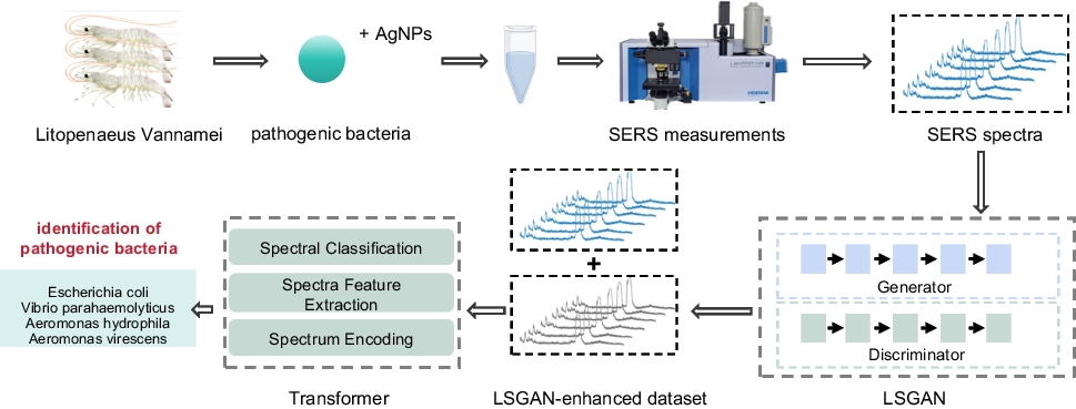
Remember me
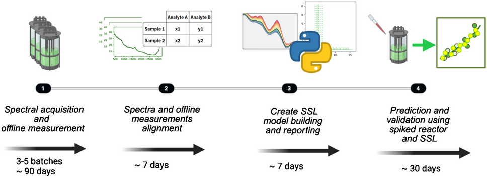
The two distinct Raman calibration methodologies employed in this manuscript together with the industry standard are illustrated in Fig. 1. The first approach, depicted in Fig. 1a and typically used in the industry, relies solely on spectral acquisition and offline analytics, necessitating multiple costly bioreactor runs to accumulate sufficient data for model development. This workflow can extend up to 6 months when accounting for the preparation of runs, sample allocation, and analysis along with signal processing. Furthermore, the data accrued for model building does not facilitate the decoupling of correlations between similarly varying analytes, resulting in suboptimal model performance. Testing and validation are often conducted with another batch that follows analogous overall trends. However, without physical spiking of the analyte of interest, model robustness may remain unachieved despite the apparent strong predictive power of the model, as the correlation between the process signal and the analyte signal has not been decoupled.
Fig. 1
Schematic representation of different workflows. a The traditional approach where in-line spectral acquisition is timely aligned with the closest offline analysis requires data from several process runs for sufficient variability. b Experimental spiking can significantly reduce the amounts of experimental processes while concomitantly removing correlation of different analytes. c In silico spiking can generate similar information-rich spectra without any additional experimental effort
The second approach, conceptualized by Romann et al., capitalizes on the practical benefits of using frozen harvest library samples, avoiding the need for live runs to acquire qualitative data and enabling analyte spiking without disrupting an ongoing culture process, as shown in Fig. 1b [35]. Although this approach yields significant time savings and improved data quality, physical spiking must be performed individually for each process. It is noteworthy that the validation of chemometric models entails a spiking experiment at the conclusion, ensuring the model’s performance.
The third approach introduces a novel in silico spiking methodology termed SSL, which further extends time savings by measuring pure compounds in water at various concentrations (Fig. 1c). This method involves integrating these spectra with measurements from actual processes to impart the necessary matrix variation for optimal model performance.
Regardless of the chosen calibration approach, all regression models should be validated through physical spiking to ensure precise model calibration and reliability. In the following chapters, the results of the SSL approaches are presented, and ultimately, a comparative analysis of the three methodologies is conducted.
Fingerprint of pure compounds in waterThe first step to generating the SSL is to measure the analytes in water at different concentrations. Figure 2 shows the Raman spectra of glucose, raffinose, lactate, ammonium, glutamate, and glutamine dissolved in water at different concentrations (0, 0.5, 1, 1.5, 2, 2.5, 3, 4, 5, 6, 7, 8, 9, 10 g/L). All spectra were normalized using the average signal between 3205 and 3215 cm−1 (near the intense symmetric O–H stretching mode of water). The water spectrum was subtracted to isolate the analytes’ contributions. In the spectra of the organic molecules (all but ammonium), two distinct regions can be observed: the lower part (up to ~ 1500 cm−1) where C–C and C-O modes appear, and the upper region (~ 3000 cm−1) where C-H and O–H modes are present.
Fig. 2
Normalized Raman spectra fingerprints of a glucose, b ammonium, c raffinose, d glutamate, e lactate, and f glutamine at 0.5, 1, 1.5, 2, 2.5, 3, 4, 5, 6, 7, 8, 9, and 10 g/L in water after subtraction of the Raman spectrum of pure water
Raffinose is a trisaccharide composed of glucose, galactose, and fructose. Although it is not normally used in cell cultures, it was selected as a worst-case scenario due to the significant overlap with glucose Raman spectra, as can be observed by comparing Fig. 2a and c. As demonstrated by Romann et al. [35], PLS models must be calibrated with spectra containing sufficient concentration variability of both analytes with overlaps. In addition, physical spiking during the test run is recommended to demonstrate that the models can properly distinguish both analytes. The measured fingerprints for the present study are in agreement with other previously published works [30, 33, 34].
To compare the feasibility of detecting these analytes using the Raman measurement scheme described in the “Material and methods” section, Fig. 3 shows the SNR for three bands of each analyte (dashed lines in Fig. 2). The linear representation of the SNR as a function of analyte concentration is provided in the supplementary information (Figure SI 1). The SNR in Raman measurements is predominantly influenced by factors such as laser power and wavelength, integration time, sample properties, detector sensitivity, and optical configuration. Optimizing these parameters enhances the Raman signal intensity and reduces background noise, culminating in improved accuracy and reliability of the measurements. Although all analytes show similar trends in SNR, the shaded regions in Fig. 2 reveal that the typical concentrations of certain analytes (ammonium, glutamate, and glutamine) in mammalian bioprocesses fall in the lower range, where SNR is below 10. In such cases, the Raman model calibration and prediction is challenging, indicated by several publications [35, 36]. Since the optimization of SNR is beyond the scope of this manuscript, we will focus on the more detectable analytes (glucose, raffinose, and lactate) hereafter.
Fig. 3
Signal-to-noise ratio (SNR) of a glucose, b raffinose, c lactate, d ammonium, e glutamate and f glutamine for each of the three peaks marked with vertical dashed lines in Fig. 2. The colors (blue, red, and orange) correspond to the vertical lines in Fig. 2. A regression line is added for each peak and analyte as a guide. The shaded area indicates the typical concentration range in mammalian bioprocesses
Synthetic spectral libraries (SSL)The Raman measurements of the different analytes in water can now be combined with representative bioprocess harvest spectra to generate SSL for modeling. Figure 4 illustrates this methodology by combining glucose measurements in water with a single harvest spectrum to simulate different glucose concentrations in the harvest. First, all spectra are normalized to the averaged intensity between 3205 and 3215 cm−1, around the O–H stretching mode of water (Fig. 4a, b). The differences between glucose concentrations are then used to determine the contribution of glucose at various concentrations (e.g., the contribution of 2 g/L glucose can be calculated as 2 g/L glucose – water, 4 g/L – 2 g/L) (Fig. 4b). Note that these contributions can lead to negative normalized intensities, as all possible combinations are performed, as stated in Eq. 2. These contributions are then added to the harvest spectrum to generate the synthetically spiked library (Fig. 4c). Finally, the spectra are processed with a first derivative Savitzky-Golay filter with a window size of 31 and a second-order polynomial before PLS regression.
Fig. 4
Overview of generation of synthetic spiked spectral libraries: a all raw Raman spectra are transformed into normalized Raman spectra. b Similarly, raw Raman spectral data from pure compounds in water were also normalized. After subtracting the signal of pure water, the normalized fingerprints of pure compounds are obtained, illustratively shown for glucose in water at 0.5, 1, 1.5, 2, 2.5, 3, 4, 5, 6, 7, 8, 9, and 10 g/L. c A single normalized Raman spectrum was synthetically augmented by adding to the normalized harvest spectrum for illustrative purposes. Then the first derivative and second-order polynomial Savitzky-Golay filter with a window of 31 points was applied. After performing the same procedure with 15 different base spectra, the synthetic spectral library (SSL) is generated that builds the basis for PLS regression
Comparison of physically and synthetically spiked Raman spectraBefore evaluating the performance of the SSL library in training a prediction model, we first compared the spectra generated in silico and the spectra from physically spiked samples. Figure 5a, c, and e show a comparison of the in silico generated spectra and the experimental spectra, whereas Fig. 5b, d, and f illustrate these spectra after preprocessing. The spectra are referenced to the base spectrum for better visualization. In Fig. 5a, 8 g/L of glucose was synthetically spiked via SSL (red dotted lines) or physically spiked (green dotted lines), respectively. These baselines are not always identical and are most likely due to experimental variations between the base and spiked measurements such as small laser variations and different temperatures during measurements. No baselines are observed in the in silico spectra as the Raman measurements in water were carefully performed to obtain consistent spectra. To better compare the spectra with different baselines, we fitted them with a third-order polynomial and subtracted it. The agreement between the spectra is quite remarkable, with only small discrepancies observed around 750 cm−1 (Fig. 5b), demonstrating that the changes in the Raman spectra due to the addition of glucose and raffinose are consistent in both water and the harvest sample. This suggests that the Raman signal response to the addition of these analytes is mainly independent of the matrix (i.e., the harvest solution), as we assume for the generation of the SSL.
Fig. 5
Comparison of physically and synthetically spiked Raman spectra. a Physically and synthetically spiked spectra referenced to the base spectrum with 8 g/L of glucose. The baseline was fitted with a third-order polynomial and removed for the physically spiked spectra. b The preprocessed Raman signal with the first derivative and second-order polynomial Savitzky-Golay filter with 31-point windows of the same spectra. c The comparison of the physically and synthetically spiked Raman spectra for 9 g/L of raffinose and d the corresponding signal after preprocessing. e The comparison of the physically and synthetically spiked Raman spectra for 4 g/L glucose and 10 g/L of raffinose and f the corresponding processed signal
Ideally, the physically and synthetically spiked Raman spectra align even before processing as illustrated in Fig. 5b for 9 g/L of raffinose, resulting in comparable corresponding signal after preprocessing (Fig. 5d). However, it seems that the observed baseline shift does not significantly impact the comparison of the physically and synthetically spiked Raman spectra, demonstrated with another baseline shift in Fig. 5c and f for the case of two spiked analytes (4 g/L glucose and 10 g/L of raffinose) and the corresponding processed signal. Therefore, the conventional preprocessing algorithms appear to be effective for baseline correction.
Apart from the visual comparison presented in Fig. 5, synthetically and physically spiked spectra can be compared in terms of their correlation structure. To ensure that PLS models calibrated with synthetic spectra preserve the correlation structure of physically spiked spectra, we computed the DModX values (see Table SI 1) for the spectra shown in Fig. 5 using two PLS models calibrated with an SSL to predict glucose and raffinose respectively (see the “Raman model comparison between physical and synthetically spiked spectra” section and Fig. 6). The results obtained are below the maximum thresholds (99th percentile of the DModX values obtained for the calibration data), indicating that the physically spiked spectra lie within the correlation structure of the PLS models calibrated with synthetic spectra. In addition, Figure SI 2 shows the same spectra projected onto the latent space of the PLS models, revealing that the synthetically and physically spiked spectra appear close together in all cases. Thus, it can be assumed that the SSL spectra should be as effective as real spectra for model calibration.
Fig. 6
a Raffinose and glucose concentrations of 15 sample points from 5 different runs used as a base for creating the SSL. b Concentrations of the 155 spectra from physically spiked harvest samples. c Concentrations of the 3585 SSL1 spectra generated by in silico spiking of glucose and raffinose independently. d Concentrations of the 204,240 SSL2 spectra generated by in silico spiking of glucose and raffinose simultaneously. e Glucose concentration predictions of the verification run using PLS models calibrated with base (blue), physically (red), and synthetically (light and dark green) spiked spectra. f Raffinose concentration predictions of the verification run using PLS models calibrated with base (blue), physically (red), and synthetically (light and dark green) spiked spectra
Raman model comparison between physical and synthetically spiked spectraTo ensure that the SSL data could be used to calibrate concentration prediction models and give results similar to those obtained with physical spiking, we tested it using the two different sets of measurements and analytes described in material and methods.
From the first dataset, 15 spectra of samples containing less than 6 g/L of glucose and less than 0.5 g/L of raffinose, as depicted in Fig. 6a, were used as the base for the SSL. Figure 6b shows the design of the experiment (DOE) matrix used during the physical spiking experiment. Figure 6 c and d indicate the concentration ranges reached by SSL1 and SSL2 generation, respectively, which differ by the addition of glucose and raffinose individually or with all different combinations possible (see Table 1 for more details). In Fig. 6e and f, the PLS models’ predictions are shown for glucose and raffinose concentrations, respectively, alongside offline measurements. To better observe the accuracy of the models, Figure SI 3 also presents the predicted versus real concentrations and residuals across the entire concentration range. The model generated from the base spectra represents the first modeling approach from Fig. 1a and failed to predict both analytes, especially raffinose. This failure can be explained by examining the concentration ranges of the calibration samples, which were nearly zero for raffinose and quite small for glucose (< 2 g/L). Additionally, since the model had not been trained on significant changes in raffinose concentration, it cannot properly distinguish between glucose and raffinose, increasing the glucose prediction when raffinose is added [35]. On the other hand, the other models produced similar results, with all being able to distinguish between glucose and raffinose and provide quantitatively accurate predictions (RMSEP < 0.4 g/L in all cases). For glucose, the model with physically spiked analytes produced slightly better results (RMSEP = 0.20 g/L) than SSL1 (RMSEP = 0.27 g/L). In contrast, for raffinose, SSL1 (RMSEP = 0.19 g/L) outperformed the physically spiked model (RMSEP = 0.37 g/L). In both cases, SSL2 produced slightly worse results than SSL1. Although the differences are likely not statistically significant, these results suggest that there is no significant improvement when generating spectra that combine the addition of both analytes.
Table 1 Number of base spectra (\(_\)) and analytes (\(_\)) used to generate the SSL. Maximum number of spectra that can be generated (physical and non-physical) when the fingerprints of the different analytes are added individually (\(_\)) or combined (\(_\)). The final number of spectra \(_\) and \(_\) are determined after removing the non-physical ones (negative concentrations)To confirm that the SSL works properly under conditions where the available spectra are fewer and less representative of the process to model but still produces similar results, a new set of models was generated for the first dataset using a completely different base set. This time, the base set contains only 5 samples from 3 different runs with > 8 g/L of glucose and 10 g/L of raffinose (see Fig. 7a), so there are three times fewer samples, less variability (3 runs instead of 5), and negative spiking becomes more relevant as starting concentrations are greater. Starting from this base set, two sets of samples were synthetically generated, expanding the concentration range to both lower and higher values (see Fig. 7c and d). In Fig. 7e, f and Figure SI 4, the predictions show similar results for the SSL1, SSL2, an physically spiked models (all RMSEP < 0.5 g/L). In contrast, the base predictions are significantly worse, especially for raffinose. This can also be explained by the fact that the concentration ranges are very small for glucose and 0 for raffinose (all base samples contain 10 g/L of raffinose).
Fig. 7
a Raffinose and glucose concentrations of 5 sample points from 3 different runs used as a base for creating the SSL. b Concentrations of the 155 spectra from physically spiked harvest samples. c Concentrations of the 1815 SSL1 spectra generated by in silico spiking of glucose and raffinose independently. d Concentration of the 165,615 SSL2 spectra generated by in silico spiking of glucose and raffinose simultaneously. e Glucose concentration predictions of the verification run using PLS models calibrated with base (blue), physically (red), and synthetically (light and dark green) spiked spectra. f Raffinose concentration predictions of the verification run using PLS models calibrated with base (blue), physically (red), and synthetically (light and dark green) spiked spectra
In the same fashion, the second dataset is composed of 15 spectra of samples containing between 4.5 and 5 g/L of glucose and less than 0.7 g/L of lactate (Fig. 8a). The DOE matrix for the physical spiking of glucose and lactate is presented in Fig. 8b. Similarly to the previous figure, Fig. 8 c and d illustrate the concentrations covered by SSL1 and SSL2 respectively, with individual or combined analytes. Predicted concentrations of glucose and lactate from the PLS models calibrated with each dataset are shown in Fig. 8e, f and Figure SI 5. Similar trends were observed across all models. The concentration ranges are too small in the base spectra to accurately predict and discriminate glucose and lactate. For glucose, this time, the SSL1 prediction (RMSEP = 0.17 g/L) outperformed the physically spiked one (RMSEP = 0.22 g/L). In contrast, for lactate, the physically spiked model gives a slightly better prediction (RMSEP = 0.18 g/L) than SSL1 (RMSEP = 0.24 g/L) and SSL2 (RMSEP = 0.34 g/L). In addition to the obvious fact that models need to be calibrated with samples containing a sufficient concentration range to produce accurate results, these findings also demonstrate that the SSL models perform similarly to the physically spiked models in two different runs and for three different analytes (glucose, raffinose, and lactate) irrespective of the initial concentrations of the base samples.
Fig. 8
a Lactate and glucose concentrations of the 15 Raman spectra used as a base for creating the two SSL. b Concentrations of the 358 physically spiked harvest samples. c Concentrations of the 3645 SSL1 spectra generated by in silico spiking of glucose and raffinose independently. d Concentrations of the 211,500 SSL2 spectra generated by in silico spiking of glucose and raffinose simultaneously. e Glucose concentration predictions of the verification run using PLS models calibrated with base (blue), physically (red), and synthetically (light and dark green) spiked spectra. f Raffinose concentration predictions of the verification run using PLS models calibrated with base (blue), physically (red), and synthetically (light and dark green) spiked spectra
Comments (0)