MR models

MR is a statistical method used to assess causal relationships between an exposure (such as a modifiable risk factor or treatment) and an outcome (such as a disease or health outcome) using genetic variants as IVs. The basic principle of MR relies on the random allocation of genetic variants at conception, which is analogous to the randomization process in a randomized controlled trial (Davies et al. 2018). This random allocation ensures that genetic variants are not influenced by confounding factors and allows for the estimation of causal effects.

The MR model typically involves three key components: (1) Genetic instruments: These are genetic variants that are associated with the exposure of interest (e.g., blood pressure, cholesterol levels) and are assumed to influence the outcome only through their effect on the exposure, i.e. excluding any horizontal pleiotropy variants. Valid genetic instruments should satisfy certain assumptions, including relevance (association with the exposure), independence from confounders, and absence of direct effects on the outcome other than through the exposure. (2) Exposure: This refers to the risk factor or treatment under investigation, which is associated with and instrumented by the genetic variants used in the MR analysis. (3) Outcome: This refers to the health outcome or disease of interest, which may be causally influenced by the exposure.

The causal model can be written as

$$\left\l} } = } + \varepsilon } \hfill \\ } = }\tau + } + } = }\tau + }\tau + } + } = }\left( }\tau + }} \right) + \varepsilon \tau + }} \hfill \\ \end } \right.$$

(1)

where y and c represent the outcome and exposure traits, respectively, and τ represents the fixed causal effects of c on y. X is the genome-wide SNP genotype matrix with dimensions n × p, where n represents the number of samples and p represents the number of SNPs. Additionally, b and u are fixed SNP effects associated with c and y, respectively. The variables ϵ and e encompass non-genetic residual effects pertaining to c and y, respectively. For simplicity, we denote \(} = }\tau + }\), representing the overall SNP effects on y, incorporating both horizontal and vertical pleiotropy.

It is important to note that the genetic covariance between the exposure variable (c) and the outcome variable (y) is influenced by various factors. Specifically, the covariance between the genetic effects associated with the exposure (b) and the genetic effects associated with the outcome (\(} = }\tau + }\)) can be decomposed into two components: \(cov\left( },}} \right) = var\left( } \right)\tau + cov\left( },}} \right)\) where \(var\left( } \right)\tau\) arises from vertical pleiotropy, and \(cov\left( },}} \right)\) represents horizontal pleiotropy.

In situations where there is no horizontal pleiotropy (i.e., using valid IVs only), the value of \(\tau\) can be estimated as \(\tau = cov\left( },}} \right)/var\left( } \right)\). This estimation can be achieved using methods such as two-stage least squares (2SLS) or inverse variance weighting (IVW), especially when weights (e.g., standard errors) are available (Burgess et al. 2013). Additionally, advanced methods such as weighted median (Bowden et al. 2016), MR-Egger regression (Bowden et al. 2015), MR-PRESSO (Verbanck et al. 2018), GSMR (Zhu et al. 2018), MR-Mix (Qi and Chatterjee 2019), contamination mixture (Burgess et al. 2020) and IMRP (Zhu et al. 2021) can be employed in MR analyses. As previously reviewed (Zhu et al. 2021; Slob and Burgess 2020; Zhu 2021), there are cons and pros among the methods.

MR-Mix (Qi and Chatterjee 2019) employs a novel approach of handling horizontal pleiotropy through a mixture modelling framework. Here, IVs are categorized into distinct subpopulations, each characterized by unique causal effects on the outcome, including their effect sizes and pleiotropic impacts. MR-Mix effectively estimates the proportion of IVs within each subpopulation along with their corresponding causal effects, facilitated by the use of maximum likelihood estimation to minimize the function \(}} - }}\tau\) where \(}}\) and \(}}\) represent the estimated effect sizes of an IV for an outcome and an exposure, respectively, and \(\tau\) is the causal effect of the exposure on the outcome. MR-Mix typically performs a two-step procedure. First, they fit a mixture model to the summary statistics obtained from GWAS data, estimating the parameters of the subpopulations and their causal effects. Second, they use these estimates to perform MR analysis, estimating the causal effect of the exposure on the outcome while accounting for horizontal pleiotropy.

Similarly, the contamination mixture model (Burgess et al. 2020) assumes that genetic variants can be classified into two distinct subpopulations: a “contaminated” subpopulation, where variants exhibit horizontal pleiotropy and influence the outcome directly, and a “valid instrument” subpopulation, where variants only affect the outcome through their association with the exposure. A likelihood function is constructed from the model, where valid IVs are assumed to have a normal distribution around the true causal effect, \(\tau\), while invalid IVs are assumed to have a normal distribution around zero. The likelihood is maximized over different values of the causal effect and configurations of valid and invalid IVs. If the assumption is satisfied, then the two sets of regression coefficients will satisfy a proportional relationship in the form \(}} = }}\tau\). The causal estimate that maximizes the profile likelihood is then determined.

IMRP (Zhu et al. 2021) is an iterative method to simultaneously conduct MR analysis and identify horizontal pleiotropy variants as invalid instruments based on GWAS summary statistics. In each iteration, IMRP applies a t-test, \(\frac}} - }}\tau }}}\left( }} - }}\tau } \right)} }}\), for each IV to determine pleiotropic IVs. By identifying pleiotropic IVs and recalculating the causal effect after excluding them at each iterative step, IMRP enables simultaneous MR analysis and detection of pleiotropic variants.

These methods offer several advantages over traditional MR methods by explicitly addressing horizontal pleiotropy, leading to more accurate estimates of causal effects, especially in the presence of pleiotropic genetic variants.

Latent outcome variable approach (LOVA) for MR using the stochastic expectation maximization (EM) steps

We employ a stochastic or simplified EM algorithm (McLachlan and Krishnan 2008; Michael and Tipping 1999; Ng et al. 2012) where instead of marginalizing the likelihood with respect to the latent variable, we iteratively impute the latent variables to facilitate the estimation of model parameters.

Suppose we know the true \(\tau\) without error. According to Eq. (1), a new set of phenotypes can be generated as follows:

$$}} = } - }\tau = } + }$$

(2)

The new phenotypes, denoted by υ, exclude the vertical pleiotropy effects (\(}\tau\)), allowing only for horizontal pleiotropy effects with residual effects. By using υ, the GWAS summary statistics will distinctly reveal which variants are not associated with the outcome, satisfying the exclusion restriction assumption, a key aspect in MR.

However, given the true \(\tau\) is unknown, we propose employing an iterative EM algorithm:

1.

Initialization: Start with initial estimates for \(\tau^\) where \(t\) is the iteration number (\(t\) = 0, 1, 2, …)

2.

Expectation (E) Step: Calculate the expected values of the latent variable \(}}^ \right)}} = } - }\tau^ = } - \left( } + }} \right)\tau^\) given the observed data and the current parameter estimates. This step involves imputing the latent values based on the observed data and the current estimates of τ. The calculation of \(}}\) should incorporate both the observed data y and the linear predictor \(\left( } + }} \right)\tau^\), representing the expected value of \(}}\) given the current estimate of τ.

3.

Maximization (M) Step: Update the parameter estimates, τ, to maximize the expected log-likelihood computed in the E-step, i.e. log-L(\(\tau\) | y, \(}}\), I) where I is the inclusion indicator for vertical pleiotropy (0 or 1). This step first involves fitting a regression model to estimate the parameter, \(\hat_\), using the imputed υ values. Then, \(\tau\) can be estimated using an IVW model, represented as \(\tau_ = \frac I_ \hat_ \hat_ se\left( _ } \right)^ }} I_ \hat_^ se\left( _ } \right)^ }}\) where Ij is the inclusion indicator with Ij = 1 if the significance criteria are met; otherwise Ij = 0 (see below).

4.

Iteration: Repeat steps 2 and 3 until convergence, where the parameter estimates no longer change significantly between iterations or a convergence criterion is met.

In the EM steps, two key parameters need to be specified by the users: the initial value for τ and the significance level used to select vertical pleiotropy variants (referred to as the inclusion indicator) in each iteration.

Initial value for τ in the EM method

In many scenarios, it is often considered reasonable to start with the assumption of no causal effect and initialize the parameter τ to 0 in the EM method. This initial value implies that there is no vertical pleiotropy variant influencing the outcome. By beginning with this assumption, the analysis starts from a neutral standpoint, which can help prevent the algorithm from being biased towards finding spurious causal relationships. Consequently, initializing τ to 0 can contribute to reducing the likelihood of encountering false positives, where associations are erroneously detected between variables that do not have a genuine causal relationship. Thus, an initial value of τ = 0 was applied for both the simulations and the real data analysis.

However, it is important to acknowledge that prior knowledge about the presence or absence of vertical pleiotropy variants and the true nature of τ can greatly inform the choice of initial values. If reliable information exists regarding specific variants that may exert vertical pleiotropy effects or if there are well-established estimates for τ based on previous research or biological understanding, it may be advantageous to use these values as the initial starting point for the EM algorithm. Incorporating such prior knowledge can potentially enhance the accuracy of the estimation process by guiding the algorithm towards more relevant regions of the parameter space.

Significant criteria for the inclusion indicator in the M step

The significance level chosen for the inclusion indicator serves as a critical determinant in the process. It sets the threshold for identifying vertical pleiotropy variants. This involves carefully assessing the statistical significance of each variant's effect on both the outcome and the exposure of interest.

To implement this criterion, variants exhibiting significant effects on the latent outcome variable (i.e., outcome corrected for vertical pleiotropy based on Eq. 2) are typically excluded from the analysis, as they may introduce bias by confounding the relationship between the exposure and outcome (exclusion restriction assumption). Similarly, variants with non-significant effects on the exposure are also excluded, as they are less likely to contribute to any genuine mediation effects (relevance assumption).

By applying these criteria, researchers can effectively filter out irrelevant genetic variants and focus only on variants that have the potential to influence the causal pathway under investigation. This approach enhances the validity and reliability of the MR analysis, ensuring that the identified genetic instruments are robust and capable of providing meaningful insights into causal relationships. As a default, we employ the following criteria: if the estimated parameter \(\hat_\) (the direct effect on the outcome) has a p-value > 0.05 and \(\hat_\) (the effect on the exposure) has a p-value < 5E− 08 then Ij = 1; otherwise, Ij = 0.

MR-LOVA based on GWAS summary statistics

In the E step for each iteration, the calculation of υ involves the following equation:

$$}}^ \right)}} = } - }\tau^ = y - \left( } + }} \right)\tau^$$

This calculation necessitates individual-level data, as also shown in Eq. (1) (i.e. y, c, X). However, the proposed method can use GWAS summary stats solely, not relying on individual level data.

Without loss of generality, assuming that SNP genotypes are column-standardized and SNP effects estimated from the outcome and exposure GWAS are standardized, the updated SNP effects based on the corrected phenotypes, υ, can be derived as

$$\hat_^ \right)}} = }}_ - \tau^ \hat_$$

and, the sampling variance of the updated SNP effects for the outcome can be expressed as

$$\begin } \left( _^ \right)}} } \right) & = \frac\left( } \right)} \left( \upsilon \right) \\ & = } \left( _ } \right) + \frac - 2\tau *} \left( \right)}} \\ \end$$

where R2 (proportion of variance in the corrected phenotype \(\left( \right)\) explained by a single genetic variant j) is typically close to zero, owing to a single genetic variant, \(var\left( \upsilon \right) = var\left( y \right) + var\left( c \right)*\tau^ - 2\tau *cov\left( \right) = 1 + \tau^ - 2\tau *cov\left( \right)\), and \(var\left( _ } \right) = \fracvar\left( y \right) = \frac\). Note that \(var\left( }}_ } \right)\) is assumed to be known from GWAS summary statistics, and cov(y,c) can be approximated as \(cov\left( }}_ , \hat_ } \right)\), assuming that correlations among genetic variants are negligible, i.e. using approximately independent SNPs after pruning or clumping (Stephens 2013). Therefore, given updated \(\hat_^ \right)}}\) and \(var\left( _^ \right)}} } \right)\), the EM algorithm can be operated.

The assumption of negligible correlations among genetic variants can be relaxed by incorporating the correlation structure among SNPs from a reference panel data (1 KG or HapMap). Following (Momin et al. 2023), the estimated regression coefficients from a multiple regression that accounts for the correlation between explanatory variables are given by \(}}^ }}\) where \(}}\) is the correlation matrix among IVs. The variance of \(}}^ }}\) is expressed as:

$$var\left( }}^ }}} \right) = diag\left[ }}}} \right)^ } \right]\left( } \right)$$

where \(var\left( \upsilon \right) = 1 + \tau^ - 2\tau *cov\left( \right)\) and \(R^ = \left( }}^ }}} \right)^ }}\left( }}^ }}} \right)\), which is not negligible due to the presence of multiple genetic variants.

Permutation

Permutation testing is often paired with the EM algorithm, particularly in scenarios where conventional statistical assumptions may not apply or when the null distribution of a test statistic is unknown. This method involves iteratively reshuffling the labels of observed data points to create a null distribution for the test statistic. By comparing the observed test statistic to the distribution derived from these permutations, one can gauge the significance of the observed result. Permutation testing offers a non-parametric approach to hypothesis testing, enabling control over the type I error rate under the null hypothesis without necessitating specific distributional assumptions. In our approach, we employ permutation by shuffling both the estimated parameter \(\hat_\) and its standard error. As expected, MRLOVA with permutation testing can substantially increase computational load, although without permutation, its efficiency remains comparable to other MR methods.

Statistical test for directional pleiotropy and InSIDE assumption violation

The proposed method, which estimates direct SNP effects (u in Eq. (1)) based on latent outcome variables (\(}}\)), facilitates tests for both directional pleiotropy and the InSIDE assumption violation.

The directional pleiotropy test is performed using a one-sample t-test to determine if the mean of u is significantly different from zero. A significant p-value indicates directional pleiotropy, while a non-significant p-value suggests its absence. This test is compared with the MR-Egger method, a standard approach for detecting directional pleiotropy.

The InSIDE assumption violation test assesses the correlation between direct SNP effects on the outcome and genetic effects on the exposure, i.e. cor(u,b). A Pearson correlation test determines if cor(u,b) significantly differs from zero. A significant p-value indicates a violation of the InSIDE assumption, whereas a non-significant p-value suggests no violation.

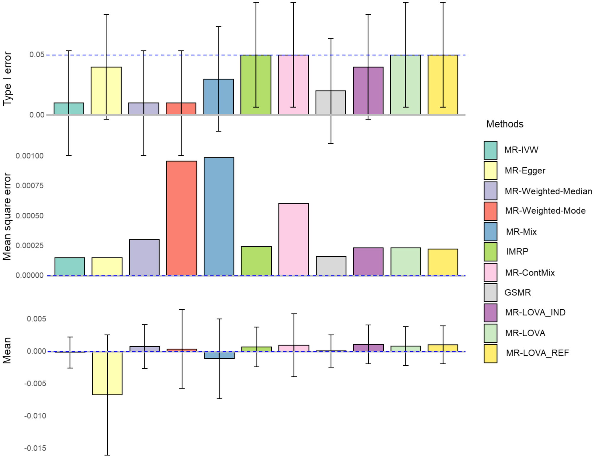
Simulation

To demonstrate the performance of the proposed method compared with existing MR methods, we conducted a simulation study. Following previous studies (Slob and Burgess 2020; Lin et al. 2021), we used four distinct scenarios, (1) no pleiotropy, (2) balanced pleiotropy, (3) directional pleiotropy and (4) pleiotropy through a confounder. The Instrument Strength Independent of Direct Effect (InSIDE) assumption holds true for all scenarios except the fourth.

We simulated data according to Eq. (1), with the additional consideration of a confounder as follows:

$$\left\l} } = } + }}} \hfill \\ } = } + } + }} \hfill \\ } = }\tau + } + } + }} \hfill \\ \end } \right.$$

where z is a confounder that is often unobserved, \(}\) represents SNP effects associated with z, \(}}\) denotes non-genetic residual effects pertaining to z, and other terms are already defined as above.

Following (Slob and Burgess 2020; Lin et al. 2021), the entries of the nxm genotype matrix X were independently drawn from a Binomial distribution B(2, fi). For each SNP i, its MAF fi was determined independently from others using a uniform distribution U(0.1, 0.3).

The IV strengths \(}\) were generated from a left-truncated normal distribution. For m = 30, IV strengths were generated from N(0, 0.1) left-truncated at 0.1. For m = 100, they were from N(0, 0.05) left-truncated at 0.05.

When considering scenarios involving pleiotropy (2–4), the details are as follows:

Scenario 2: Balanced pleiotropy and InSIDE satisfied, where pleiotropy effects \(}\) were generated independently from N(0,0.15) and \(}\) = 0;

Scenario 3: Directional pleiotropy and InSIDE satisfied, where \(}\) were generated from N(0.1, 0.075) and \(}\) = 0;

Scenario 4: Directional pleiotropy and InSIDE violated, where \(}\) were generated from N(0.1, 0.075) and \(}\) were generated from U(0; ɵ).

\(}}\), \(}\), \(}\) were generated from N(0, 1) independently.

The summary data for genetic associations were calculated for the exposure and the outcome on non-overlapping sets of individuals, each consisting of n individuals. For scenarios (2) and (3), τ was varied between 0 and an expected value of 0.2 when both the outcome and exposure are scaled (i.e., the true τ under unscaled traits is τ scaled multiplied by the standard error of the outcome divided by the standard error of the exposure). The investigation included different proportions of invalid IVs: 0, 0.3, 0.5, and 0.7, with sample sizes for exposure and outcome set at 10,000 or 50,000. For scenario (4), We investigated various levels of correlated pleiotropy effects by varying ɵ across three values: 0.1, 0.4, and 0.7.

Real data analysis

We applied the proposed method (MR-LOVA) to analyse publicly available GWAS summary-level data to explore causal relationships underlying variety of exposure-outcome pairs of interest. We assessed data for coronary heart disease CAD) (Nikpay et al. 2015) as the outcome and analysed its relationship with blood lipids (Willer et al. 2013), blood pressure (Neale n.d.) as exposures. We selected these pairs based on sample sizes, number of instruments, and existing evidence from epidemiological and recent MR studies (Qi and Chatterjee 2019; Zhu et al. 2021; Xue et al. 2021; Lin et al. 2021; Mounier and Kutalik 2023).

In addition, we analysed the relationship between BMI (Yengo et al. 2018) as an exposure and MetS (Lind 2019; Walree et al. 2022) as an outcome. Although obesity and MetS are genetically correlated (Walree et al. 2022; Amente et al. 2024), they are distinct phenotypes. For instance, some individuals are metabolically healthy despite being obese, while others are metabolically unhealthy despite having a normal weight (Bluher 2010). This distinction makes it particularly interesting to explore whether obesity directly causes MetS (Despres 2006; National Heart and Institute n.d.; Grundy 2004). Pairs with high genetic correlations, such as BMI and MetS, serve as a valuable case for comparing methods, as they are prone to horizontal pleiotropy, which mirrors the simulation scenario 4, where the InSIDE assumption is violated. While the causal relationship between obesity and MetS is an important question, our primary focus here is on comparing methodological approaches.

For MetS, we extracted GWAS summary data for both binary and continuous outcomes. The binary outcome is referred to as MetS, and the continuous outcome is termed MetS score. MetS (binary) was defined based on the International Diabetes Federation criteria (Alberti et al. 2009), with individuals classified as having MetS if they met three or more of the following criteria: central obesity (WC ≥ 88 cm in females and ≥ 102 cm in males), elevated fasting triglycerides (TG) levels (≥ 1.7 mmol/L or medication for elevated TG), reduced high density lipoprotein cholesterol (HDL-C) (< 1.29 mmol/L in females and < 1.03 mmol/L in males or medication for reduced HDL-C), elevated blood pressure (systolic blood pressure/diastolic blood pressure (SBP/DBP) ≥ 130/85 mmHg), and elevated fasting glucose (≥ 5.6 mmol/L or medication for elevated glucose). The MetS score, a weighted sum of scores from the five components based on the genomic structural equation modelling (Grotzinger et al. 2019), captures genetic correlations and shared genetic variance among the components (Walree et al. 2022). MetS scores provide potentially richer information than the binary MetS classification (Walree et al. 2022; Graziano et al. 2016). GWAS summary data for MetS score was obtained from the Complex Trait Genetics Lab (CTG) (https://ctg.cncr.nl/software/summary_statistics), which contains 461,920 valid subjects of European ancestry.

Genetic correlation between the traits were estimated using LD regression score (Bulik-Sullivan et al. 2015). For MR analysis, we only selected SNPs as potential instruments if they reached genome-wide significance (p-value < 5 × 10−8) in the exposure GWAS. Furthermore, we used LD clumping with an r2 threshold of 0.1 and a window size of 500 kb to select a set of independent instruments for each trait.