TV-EM and modified-BSREM were compared with RAREM. In this study, scatter, attenuation, and collimator aperture corrections were not used to compare the differences between image reconstruction methods.

In SPECT, the projection data follows the Poisson distribution \(P\left( }|}\right)\).

$$\begin P(}|}) = \prod ^M _ \left[ \frac _ C_ x_j \right) }^} \exp \left( -\sum ^ _ C_ x_j \right) \right] , \end$$

(1)

where, \(x_j\) is the radioactivity concentration in the j-th pixel of matrix size \(N^2\), \(y_i\) is the projection data in the i-th projection data of M, and \(C_\) is the detection probability from the j-th image pixel to the i-th projection data. The ML method estimates \(}\) maximizing the logarithm of Equation (1), which is the log-likelihood function \(L\left( }\right)\), as follows [17]:

$$\begin L\left( }\right) = \sum ^M _ \left[ y_i \ln \left( \sum ^ _ C_ x_j \right) - \sum ^ _ C_ x_j \right] . \end$$

(2)

The MAP-EM algorithm, based on Bayes’ theorem, maximizes the log-likelihood function (2) and the prior function. Bayes’ theorem is as follows:

$$\begin P\left( }|}\right) = \frac}|}\right) \cdot P\left( }\right) }}\right) }, \end$$

(3)

where, \(P\left( }\right)\) is the prior function and is assumed to be a Gibbs distribution [4].

$$\begin P\left( }\right) \propto \exp \left( -\eta U\left( }\right) \right) , \end$$

(4)

where, \(U\left( }\right)\) is the energy function, and \(\eta\) is a regularization parameter. Using Equations (2), (3), and (4), the reconstruction problem of the MAP-EM algorithm is the logarithm of the posterior probability shown in the following equation:

$$\begin \arg \max _}} \ln P\left( }|}\right)&= \arg \max _}} \left\}\right) + \ln P\left( }\right) \right\} \\&= \arg \max _}} \left\ \left[ y_i \ln \left( \sum ^ _ C_ x_j \right) - \sum ^ _ C_ x_j \right] - \eta U\left( }\right) \right\} .~~ \end$$

(5)

The MAP-EM algorithm is derived to solve problem (5) and is shown in the following equation [3]:

$$\begin x ^ _j = \frac C_ + \eta \frac U\left( }\right) \bigg |_} = } ^k}} \sum ^M _ \frac} _ C_ x ^k _n}, \end$$

(6)

where, k is the number of main iterations. In the TV-EM algorithm, the TV norm is used for \(U\left( }\right)\), and is expressed as follows [4]:

$$\begin U_} \left( }\right) = \sum _ \sqrt - x_ \right) ^2 + \left( x_ - x_ \right) ^2}, \end$$

(7)

where, s and t are the pixel numbers in the horizontal and vertical directions of the two-dimensional image, respectively. As the TV norm is not a differentiable function, an approximate formula for the partial derivative of the TV norm by \(x_\) was used.

$$\begin \frac}\left( }\right) }}&= \frac - x_} - x_\right) ^2 + \left( x_ - x_\right) ^2 + ^2}} \\&+ \frac - x_} - x_\right) ^2 + \left( x_ - x_\right) ^2 + ^2}} \\&- \frac + x_ - 2x_} - x_\right) ^2 + \left( x_ - x_\right) ^2 + ^2}}, \end$$

(8)

where, \(\varepsilon\) is an artificial parameter to ensure the differentiability around a point where \(U\left( }\right) =0\) and usually set to a small value. A previous study mentioned that \(\varepsilon\) should be set to 1% or less of the expected maximum value of \(}\), and that TV-EM is not sensitive to \(\varepsilon\) [4]. Therefore, in this study, \(\varepsilon\) was set to 0.001.

BSREM is a relaxed type of regularization reconstruction method, which is an extension of RAMLA to the regularized case and is derived by differentiating \(L\left( }\right)\) and \(P\left( }\right)\) [9]. The BSREM algorithm is expressed as follows:

$$\begin&x ^ _j = x ^ _j + \lambda _k x ^ _j \sum _ C_ \left( \frac _C_x ^ _j} - 1\right) , \end$$

(9)

$$\begin&x ^ _j = x ^ _j + \lambda _k x ^ _j \eta \frac U\left( }\right) \Big | _} = }^} , \end$$

(10)

$$\begin&x ^ _j = x ^ _j , \end$$

(11)

where, \(\lambda\) is the relaxation parameter, q is the number of sub-iterations, \(S_q\) represents all elements in the q-th sub-iteration, and Q is the total number of sub-iterations. As the name implies, the modified-BSREM is a modified version of the BSREM proposed to converge to global solutions under realistic conditions [10]. In the modified-BSREM, the update formula and relaxation parameters are controlled to not exceed the upper and lower bounds to comply with the constraints, and non-negative value processing is included in the algorithm (Table I and II in [10]). The relaxation parameter of the modified-BSREM is given by:

$$\begin \lambda _k=\frac, \end$$

(12)

where, \(\lambda _0\) is the initial value of the relaxation parameter, and \(\gamma\) is the rate for decreasing the relaxation parameter \(\lambda\) for each main iteration k. The user is required to experimentally set \(\lambda _0\), \(\gamma\), Q, and \(\eta\) to use the modified-BSREM appropriately. In the modified-BSREM, since the one of the conditions for convergence to optimal solution is \(\sum ^ _ \lambda _k =\infty\), a reconstruction is almost independent of \(\gamma\) [10]. We verified this in a preliminary experiment, and the influence of \(\gamma\) on reconstruction is small when \(\gamma\) is small enough. Therefore, in this study, \(\gamma\) was set at 0.1 and Q included at least three projections in each subset [10].

The image reconstruction method of RAREM was derived by referring to RAMLA and DRAMA using MAP estimation [1,2,3,4, 9]. In RAMLA,

$$\begin g_q \left( }\right) = \sum _ \left[ y_i \ln \left( \sum _ ^ x_j} \right) - \sum _ ^ x_j} \right] , \end$$

(13)

$$\begin x_j ^ = x_j ^ + \lambda _k x_j ^ \frac}\right) }}}, \end$$

(14)

are derived by incorporating the row-action algorithm into the ML estimation in Equation (2), where, \(g_q \left( }\right)\) is the log-likelihood function \(L\left( }\right)\) in the row-action algorithm. Equation (14) is equivalent to Equation (9) in the BSREM algorithm. The goal of RAREM is to maximize Equation (5), which is derived from the logarithms of posterior probability \(P\left( }|}\right)\). Therefore, \(g_q\left( }\right)\) can be rewritten as

$$\begin g_q \left( }\right) = \sum _ \left[ y_i \ln \left( \sum _ ^ x_j} \right) - \sum _ ^ x_j} \right] - \eta U\left( }\right) \end$$

(15)

and differentiated with respect to \(x_j\) to maximize it, the RAREM algorithm is derived as follows:

$$\begin & x ^ _j = x ^ _j + \nonumber \\ & \lambda ^ x ^ _j \left\ C_ \left( \frac _C_x ^ _j} - 1\right) - \eta _k \frac U\left( }\right) \Big | _} = }^}\right\} , \end$$

(16)

$$\begin & x_j ^ = x_j ^. \end$$

(17)

In RAREM, the number of subsets is set to the maximum, as in RAMLA and DRAMA, and each parameter is calculated automatically considering the objective structure and acquisition conditions. In this study, the TV norm in Equation (8) is used for regularization term \(\partial U_} \left( }\right) /\partial x_\). The regularization parameter \(\eta _k\) is calculated by the following equation:

$$\begin \eta _k = \frac \times \left\}\right) + 0.3 \times A_} \right\} , \end$$

(18)

$$\begin A_} = \max \left\ }} }, 0 \right\} , \end$$

(19)

$$\begin A_} = \max \left\ \left( \frac \times \frac\right) , 0 \right\} , \end$$

(20)

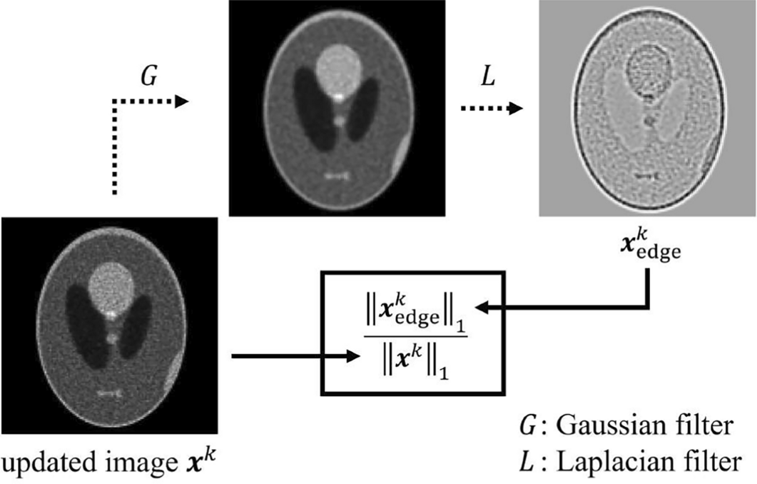
where, \(M_}\) is the number of projections that satisfy the Nyquist-Shannon sampling theorem, and T is the total number of counts. \(\max \left( a,b\right)\) indicates the calculation that selects a higher value a or b. \(A_}\) can be thought of as the term relating to the number of projections, and \(A_}\) as the term relating to the counts. \(E_k\) is the evaluation term of the object structure. A schematic of the calculation of \(E_k\) is shown in Fig. 1, \(E_k\) is calculated using the following equation:

The schematic calculation of \(E_k\). \(E_k\) is the ratio of the sum of the absolute pixel value of the updated image \(}^k\) to that of the edge image \(}^k _}\)

$$\begin E_k = 100 \times \frac}_} ^k\big \Vert _1}}^k\big \Vert _1}, \end$$

(21)

$$\begin } ^k _} = \left( } ^k \otimes G \right) \otimes L, \end$$

(22)

where, \(\big \Vert }_} ^k\big \Vert _1\) is the L1 norm of the updated image processed by the Gaussian filter G and Laplacian filter L for the calculation of \(E_k\) only. In this study, the standard deviation \(\sigma\) of the Gaussian filter, with a kernel size of \(5 \times 5\), was set to the following equation:

$$\begin \sigma = 0.4 \times \left\ \left( \frac\right) \right\} \times \left( \frac\right) ^. \end$$

(23)

All of the pixel values of the initial image \(}^0\) were 1.0, but the image reconstructed by DRAMA was used for \(}^0 _}\) with \(\text = \left\lfloor \frac}} \right\rfloor +1\), where \(\lfloor \cdot \rfloor\) is a floor function.

The relaxation parameter \(\lambda ^\) is calculated by the following equation:

$$\begin \lambda ^ = \frac \times \frac }}}} \times \frac}}. \end$$

(24)

If the acquisition condition was \(M_}<M\), \(M_}/M\) is set to 1.0. Equation (24) can be devided into three factors. The initial factor is the width of the decrease in \(\lambda\) utilized in DRAMA, with \(\gamma\) generally set to 1.0 [2]. \(\beta _0\) is the parameter calculated by the average of geometrical coefficients among the projection lines in PET and approximately balances the noise propagation from all subsets at the end of each main iteration [2]. In other imaging modalities, \(\beta _0\) is calculated by approximate expression [18, 19].

$$\begin \beta _0 \approx 0.72 \times \frac}} \frac}}, \end$$

(25)

where, \(s_}\) is defined as the FWHM of the post-smoothing filter, however, since this study did not use the post-smoothing filter, the TV norm is assumed to be the Gaussian filter with \(\sigma = 1.3\). \(s_}\) was calculated by the following equation, which relates FWHM to standard deviation \(\sigma\):

$$\begin \text = 2 \sigma \sqrt, \end$$

(26)

resulting in \(s_} = 3.06\). The second factor in Equation (24) is the factor taking into account the number of projections. The third factor in Equation (24) is to satisfy the non-negativity constraint in the RAREM algorithm, which contributes to the fact that RAREM does not require non-negative constraints and the process of replacing negative value with non-negative value in effect. To derive this factor, Equation (16) is transformed:

$$\begin & x^ _j = \\ & x ^ _j \Bigg [ 1 + \left. \lambda ^ \left\ C_ \left( \frac _C_x ^ _j} - 1\right) - \eta _k \frac U\left( }\right) \Big | _} = }^}\right\} \right] . \end$$

(27)

As \(x ^ _j\) is a non-negative value, we need to consider only the inside of the square brackets in Equation (27). Moreover, since \(\lambda ^\) is also a non-negative value, we consider when the inside of the curly brackets in Equation (27) is a minimum value. The minimum value for the first term inside the curly brackets is \(-1\), because both \(C_\) and \(y_i\) are also non-negative values. The minimum value for the second term inside that is when \(\frac U\left( }\right) \big | _} = }^}\) is a maximum value \(V_}\). From the above, we can obtain the following inequality to ensure that \(x ^ _j\) is a non-negative value:

$$\begin 1+\lambda ^ \left( -1-\eta _k V_}\right) > 0. \end$$

(28)

Finally, inequality (28) is transformed, and the third factor in Equation (16) is obtained using the following inequality:

$$\begin \lambda ^ < \frac}}. \end$$

(29)

The \(V_}\) of the partial derivative of the TV norm (8) is \(2+\sqrt\), and the proof of this is shown in Appendix A.