DatasetBone scan images

The data used in this experiment were obtained from the Department of Nuclear Medicine, Gansu Provincial Cancer Hospital, using the osteophilic 99mTc-MDP drug to detect bone lesions, and the image acquisition was performed by a Siemens SPECT ECAM imaging device. The resolution of the SPECT images was 256 (pixels) × 1024 (pixels), and the pixel pitch was 2.26 mm. The acquisition time for each whole-body bone scan image is 10–15 min. Unlike natural images, which have a pixel range of 0–255, each SPECT image is a 256 × 1024 matrix of values consisting of 16-bit unsigned integers, where each value represents the radiation value of a radioactive element. A patient examined by bone scanning produces two images in the anterior and posterior positions. After screening, the dataset used in this experiment contains 286 SPECT images.

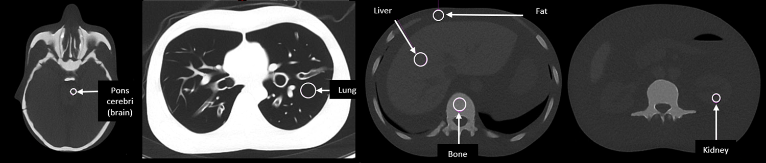
The thoracic region is a common site for bone metastases in lung cancer, so we cropped the image to 256 × 256 pixels using the method in [13], and only the thoracic region was retained in the cropped image.

Image labelling

SPECT image segmentation is a supervised task that requires accurate and reliable lesion segmentation annotation maps as the gold standard. To facilitate the labelling of lesions, this experiment used the SPECT image annotation system developed by our team based on LabelMe [14], an open-source online tool released by MIT. Three physicians with many years of clinical experience in nuclear medicine in the group manually labelled the areas of bone metastasis lesions, and the labelling information included custom symbols, disease names or body parts to ensure that the labelling information was correct. During the labeling process, each doctor annotates each image and discusses regions of inconsistency among the three annotators, and then votes to determine the final labeling result. After the annotation is completed, each image corresponds to a real segmentation map.

As shown in Table 1, in this experiment, we divided the dataset according to the ratio of training set: test set: 3, using 200 images as the training set and 86 as the test set. When dividing the dataset, we strictly placed the anterior and posterior images of the same patient into the same type of dataset because they will show similarity. There are 118 patients’ data contained in the training set and 53 patients’ data contained in the test set.

Table 1 Overview of the dataset used in this workOverall architecture

In SPECT bone scan images, lung cancer lesions often exhibit a wide range of scale variation due to individual patient differences and the unpredictable distribution of cancer lesions. Additionally, other conditions such as inflammations, fractures, and residual radionuclide drugs in the spine may create regions of radionuclide hyperconcentration similar to those of metastatic bone lesions. These regions, with similar characteristics and wide-scale variations, present significant challenges for the accurate segmentation of lung cancer metastatic bone lesions. To address these issues, our proposed model focuses on enhancing multi-scale feature detection capabilities.

Specifically, we employ a generative adversarial network with an encoder-decoder architecture for the generator. Within the encoder, we integrate a cascade dilated convolution (CDC) module to enhance multi-scale feature extraction, while augmenting receptive fields through a multi-scale feature extraction (MSFE) module. In the decoder, we replace U-Net’s conventional convolution with a residual multi-scale (RMS) module [15], thereby expanding receptive fields without introducing additional parameters. To mitigate semantic loss from encoder downsampling, we employ an input image pyramid strategy. Additionally, we incorporate deep supervision and a multi-layer convolutional discriminator to refine segmentation, as proposed by Xue [16]. This approach enhances the model’s multi-scale segmentation capabilities via backpropagation.

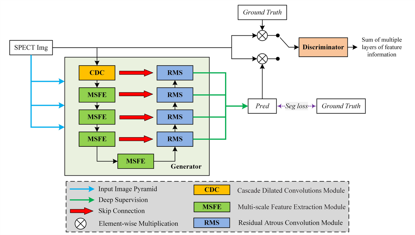
Figure 1 illustrates the workflow of the proposed segmentation method. The generator network generates a set of predictions based on the original image. These predictions are then combined with the original image and the labeled image (i.e., ground truth) using an element-wise multiplication operation. The combined image is subsequently fed into the discriminator network to determine its authenticity, resulting in a multi-scale L1 loss.

Fig. 1

The workflow of the adversarial learning-based segmentation method for automatically identifying and delineating metastasis lesions in SPECT bone scintigrams. The generator integrates a MSFE module, CDC, and deep supervision to enhance sensitivity to lesions of varying scales, while the discriminator employs a multi-scale L1 loss computed over paired image–mask inputs to guide structure-aware learning

The generator and discriminator networks are elaborated below.

The generator network

To enable the model to focus on size-varied lesion objects in low-resolution bone scintigrams, we integrate three key techniques: the CDC module, MSFE module, and RMS module, to propose a lesion-sensitive generator. The structure of the generator network is depicted in Fig. 2.

Fig. 2

The structure of the proposed generator

As illustrated in Fig. 2, the proposed generator network follows the encoding-decoding architecture, where average pooling and bilinear interpolation are used for the encoding and decoding tasks, respectively.

Cascade dilated convolution (CDC)

As shown in Fig. 3, the original input image is first processed by a CDC block. Unlike the U-Net network, which uses a 3 × 3 convolution kernel, our CDC block employs three different dilation rates (i.e., d = 1, 2, 4) to capture the size-varied lesions. The duplicate configuration of CDC blocks allows the model to extract richer features of bone metastasis lesions.

Fig. 3

The structure of the CDC block used in the proposed generator network

The dilated convolutions used can effectively reduce the computational burden often associated with conventional convolutions using large kernels. The dilation rates of d = 1, 2, 4 are determined according to the design of hybrid dilated convolution (HDC) [17], which are robust enough to cope with the gridding effect.

After each dilated convolution, there is a batch normalization (BN) layer [18] and a ReLU function layer. Therefore, the reception fields for all six dilated convolution layers are 3, 7, 15, 17, 21, and 29 (see Table 2).

These values are calculated based on Eq. (1), and for clarity, we summarize them in Table 2 to provide an intuitive illustration of how different dilation rates affect the receptive field size across the CDC block.

This summary helps readers easily grasp the cumulative impact of dilation rates and their stacking order without the need for manual computation. The reception field, rf is calculated according to Eq. (1).

$$\:r_=\left\1&\:i=1\\\:ks+\left(ks-1\right)\times\:\left(d-1\right)&\:i=2\\\:ks+\left(ks-1\right)\times\:\left(d-1\right)+s\times\:\left(r_-1\right)&\:i>2\end\right.\:$$

(1)

Table 2 An illustration of calculating the reception fields with the input and its corresponding parameters in each dilated convolution layer

In Eq. (1) and Table 2, all convolutional layers are configured with fixed parameters: kernel size ks = 3 × 3, channels c = 64, stride s = 1. The variable parameters– padding p and dilation rate d −− are explicitly listed in Table 2.

Multi-scale feature extraction (MSFE)

The MSFE block is used from the 2nd to 5th layers in the generator network. An MSFE block consists of a cascade residual atrous convolution (CRAC) module and a reception field block (RFB) [19] module, depicted in Fig. 4. The “Conv” in the figure represents a convolutional module consisting of a “Conv-BN-ReLU” three-layer structure.

As shown in Fig. 4, a CRAC module is created by adding a residual connection path [20] to the CDC block to alleviate the vanishing gradient problem and accelerate convergence. Additionally, the RFB module of the MSFE block adopts the design of the Inception network [21]. This multiple-branch configuration helps the model to focus on lesions of different sizes.

Fig. 4

The structure of the MSFE block used in the proposed generator network. Each Conv module consists of a three-layer structure of Conv + BN + ReLU

Specifically, the CRAC module consists of six cascaded convolutional modules, where each convolutional module has a convolutional kernel size of 3 and expansion rates of 1,2,4,1,2,4, in that order. To alleviate the problem of gradient vanishing and accelerate the convergence of the model, residual connectivity is added between the first and the third, and the fourth and the sixth layers, respectively. The RFB module consists of a three-branched structure connected in parallel with a residual path. The equivalent convolutional kernel sizes of the three branches are, in order, 1,3,5. Convolutional layers with dilation rates of 1, 3, and 5 are added sequentially after the corresponding branches. Finally, the results from the three branches are summed element-wise with the residual paths and the CRAC module outputs, then processed by a ReLU activation function to obtain the final results of the MSFE module.

By integrating the multi-scale and dilated convolutions in parallel, our MSFE block can learn fine-grained features of the size-varied lesions from SPECT bone scintigrams. Using MSFE blocks in different layers enables the model to extract hierarchical features, including lower boundary and texture information, as well as higher semantic information.

Residual multi-scale module (RMS)

To enable the decoder to better predict lesion information at different scales, three cascaded dilated convolution-BN-ReLU structures [15] are used instead of the double-layer convolution in the U-Net model.

As shown in Fig. 5, the dilation rates of the three dilated convolutions in the RMS module are 1,2, and 4, respectively, with residual connections added after the first and third layers. Unlike the two-layer convolution in the classical U-Net decoder, the dilated convolution expands the reception field without increasing the number of parameters. This enables the network to obtain more semantic information from lower resolution feature maps, reduces computational effort, and improves the model’s ability to accurately segment targets at different scales.

Fig. 5

The structure of the RMS block used in the proposed generator network

Input image pyramid

During the encoding stage, the repeated use of down-sampling and convolutions may result in information loss. This is problematic for the SPECT scintigrams with very low spatial resolution. To cope with this issue, an input image is halved using an averaging pooling operation at each layer. This reduced image is then concatenated with the output feature map of the previous layer (i.e., channel concatenation) to compensate for possible information loss.

Specifically, three images with sizes of 1/2, 1/4, and 1/8 of the original image are concatenated after the first, second, and third layers, respectively, as shown in Fig. 2 to provide compensation for feature maps.

Deep supervision

A typical observation is that a deeper network offers better performance but can lead to the vanishing gradient problem during model training. To address this, a deep supervision mechanism [22] is used to supervise each layer of the feature reconstruction process, providing feedback through a loss function to optimize training.

During the decoding stage, except for the last layer, a 1 × 1 convolution is used to reduce the number of channels to 1 in each layer. Bilinear interpolation is then utilized to rescale the feature map to the same size as the input. Finally, a sigmoid function is applied in each layer to limit the pixel value to a range of 0 to 1. During the training process, the four predicted segmentation maps output by the segmentation network are compared with the real segmentation maps to compute the adversarial loss and segmentation loss, respectively. These losses are then summed to obtain the overall adversarial loss and segmentation loss.

With the deep supervision strategy, supervisory signals are added to different layers of the segmentation network decoder, allowing feedback and gradient updates at various stages. By making predictions at multiple layers, the network can utilize both local and global information, thus improving the ability to perceive structures at different scales and enabling the model to produce robust segmentation results for targets of varying sizes.

The discriminator network

Unlike traditional generative adversarial networks (GANs), in this work, we use the authenticity label map and multiply it by the corresponding elements of the original map to obtain the original map mask. This mask is then fed into the discriminator, and the L1 loss between the two is calculated as the adversarial loss for both the generator and the discriminator.

We use the discriminator network proposed in [16], as shown in Fig. 6. The discriminator extracts different levels of features through a multilayer convolutional structure, then flattens and weights them into a one-dimensional tensor to obtain the final result. During training, the original image masks corresponding to the predicted and real segmentation results are fed into the discriminator to obtain the respective sums, and then the L1 loss between them is calculated as the adversarial loss. By fusing features from different levels, the discriminator can capture the long and short distance spatial relationships between pixels at multiple scales, improving the perception of lesions at different scales.

In the traditional GAN network, the discriminator outputs the probability that the input label is true. However, in our dataset, experiments show that this scheme makes the discriminator too strong to form the correct training feedback to the generator, leading to an unstable or even failed training process. Moreover, simple one-dimensional probability values cannot provide stable and sufficient gradient feedback to the network. Therefore, in the discriminator, we choose to output the weighted sum of the output results of the input data at different convolutional layers, thus obtaining the overall representation of the original image mask at different scales. On the SPECT image, the multi-scale L1 loss achieves better segmentation results.

Fig. 6

The structure of the discriminator

Loss function

For the adversarial learning-based segmentation framework, the overall objective is to maximize the generation capability of the generator G, while minimizing the discriminative ability of the discriminator D. The joint optimization objective is expressed as:

$$\:\zeta\:\left(G,D\right)=L\left(G\right)+L\left(D\right)\:$$

(2)

Here, L(G) represents the generator loss, and L(D) denotes the discriminator loss. The detailed formulation of each component is given below.

(1)

Generator Loss L(G)

The generator loss L(G) comprises two components: a segmentation loss Lseg(G) and an adversarial loss Ladv(G):

$$\:L\left(G\right)=_\left(G\right)+_\left(G\right)\:$$

(3)

where α and β are weighting coefficients to balance the two terms.

Segmentation loss

To effectively guide the segmentation network, we adopt the Dice loss, which is widely used in medical image segmentation. The segmentation loss is averaged over four decoding layers and defined as:

$$\:_\left(G\right)=\frac^}\left(1-Dice\left(_,gt\right)\right)\:$$

(4)

where yi denotes the segmentation prediction at the i-th layer, and gt is the corresponding ground truth.

Adversarial loss

The adversarial component encourages the generated segmentation to be indistinguishable from the ground truth when fused with the input image. It is defined as.

$$\:_\left(G\right)=\frac^|D}\left(_\times\:image\right)-D\left(gt\times\:image\right)|\:$$

(5)

(2)

Discriminator Loss L(D)

The discriminator aims to distinguish between real (ground truth) and fake (generated) segmentation masks. Its loss is formulated as:

$$\:L\left(D\right)=_\left(D\right)=1-\frac^|D}\left(_\times\:image\right)-D\left(gt\times\:image\right)|\:$$

(6)

Experimental setup

We trained and tested the model using a PC with a 15 vCPU AMD EPYC 7543 32-core processor and A40 (48GB) GPU to meet the model’s computational power requirements. The experiments were implemented and executed using the PyTorch 1.13.0 framework. The model training parameters are shown in Table 3.

Table 3 Parameters of the proposed model

When generating predictive labels, a threshold of 0.5 was uniformly specified, where pixels greater than or equal to 0.5 were categorized as the foreground of the lesion and pixels less than 0.5 were categorized as the background.

The trained model is run 5 times on the training subset to minimize the effect of randomness. For each metric defined above, the final output of the model is the average of the results of the 5 runs. The experimental results reported in the following sections are averages unless otherwise stated. For this experiment, we set the value of the random seed to 42.

Evaluation metrics

This experiment uses Dice Similarity Coefficient (DSC), precision and recall as evaluation metrics. The definitions are given in Eqs. (7)–(9).

$$\:Precision=\frac\:$$

(8)

where TP denotes true positive, TN denotes true negative, FP denotes false positive and FN denotes false negative. In this paper, the evaluation metrics are reported as the mean ± standard deviation.