Anatomy variations

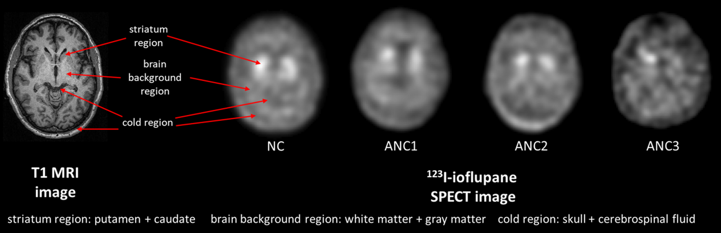
First, patients with both T1-weighted MRI and DAT SPECT data were identified from the Parkinson’s Progression Markers Initiative (PPMI) [20] database. A visual assessment was then performed on their MRI and SPECT images to exclude cases with truncation artifacts. After this screening process, a total of 200 patient datasets (age: 32–84 years, 119 males) were collected for further analysis. Based on the features from clinical DAT SPECT images, three primary regions, i.e., the high-uptake striatum region, the medium-uptake brain background region including gray and white matter, and the no-uptake cold region including skull and cerebrospinal fluid, were modeled in our phantoms (Fig. 1). The striatum region comprises 4 compartments, i.e., the left and right putamen and caudate. According to Owens-Walton et al. [21], there is only a slight volume difference (< 10%) in the striatum region across various PD stages. Vasconcellos et al. [22] also suggested that there is no significant difference in terms of volume of the caudate and putamen between PD and control groups. Thus, in this study, while we modeled the anatomical variations of the striatum, we did not account for the volume difference of the striatum between different PD stages.

We used FMRIB Software Library (FSL) [23] Version v6 (2018) to segment the MRI images. Within FSL, the model-based segmentation tool FIRST [24] was firstly used to segment left and right putamen and caudate from different T1 MRI data. The Functional MRI of the Brain’s Automated Segmentation Tool was utilized to segment gray matter, white matter and cerebrospinal fluid [25]. The outer skull surface was delineated by using Brain Extraction Tool [26]. To generate more anatomical variations, we randomly paired the striatum region and the combined background region (including the brain background and cold regions) from different patients to form a new brain phantom. To ensure the unity of the coordinates of the paired structures, we first aligned the three-segmented regions from the same MRI images by rigidly registering the striatum region to the reference striatum model of FIRST, and the resultant transformation matrix was applied to the corresponding brain and cold region (Fig. 2) using Elastix [27].

Fig. 1

Brain regions contribute to image contrast on DAT SPECT in different PD stages according to SPECT VI assessment scheme are indicated from sample MRI images. NC: Normal category; ANC1: Abnormal category 1; ANC2: Abnormal category 2; ANC3: Abnormal category 3

Activity distribution

In clinical practice, DAT SPECT images for the preliminary diagnosis of PD are commonly evaluated using the SPECT Visual Interpretation (VI) assessment scheme (Fig. 1) [28]:

1)

Normal category (NC): two symmetric comma- or crescent-shaped focal regions of activity.

2)

Abnormal category 1 (ANC1): uptake in putamen of one hemisphere absent or greatly reduced.

3)

Abnormal category 2 (ANC2): uptake absent in the putamen of both hemispheres.

4)

Abnormal category 3 (ANC3): uptake absent in the putamen of both hemispheres and greatly reduced in one or both caudate nuclei.

We then collected corresponding 123I DAT SPECT images and their striatal binding ratios (SBR = mean count in target striatum region/mean count in reference brain background region-1) for both left and right putamen and caudate, based on the previously selected 200 MRI data from the PPMI database. 99mTc DAT SPECT data of 100 patients with suspected PD symptoms (aged 35–87 years, 55 males) were also retrospectively collected in 2016 from Show Chwan Memorial Hospital under the local ethics approval (SCMH_IRB Number, 1311110704). All DAT SPECT images were categorized into different VI categories by a nuclear medicine physician with 11-year experience. For 123I, there were 20% NC, 43% ANC1, 24% ANC2, and 13% ANC3 patients, while there were 31% NC, 40% ANC1, 16% ANC2, and 13% ANC3 patients for 99mTc. For 123I, the SBR of the caudate ranged from 1.53 to 4.24 (2.66 ± 0.48), 0.63–3.76 (2.16 ± 0.60), 0.86–3.17 (1.89 ± 0.53) and 0.38–2.72 (1.48 ± 0.61) for NC, ANC1, ANC2 and ANC3 respectively, while for the putamen, SBR ranged from 0.73 to 3.04 (1.83 ± 0.43), 0.31–3.06 (1.08 ± 0.57), 0.25–2.70 (0.75 ± 0.36), and 0.12–1.58 (0.64 ± 0.30) respectively. Additionally, for the non-symmetric uptake pattern in ANC1 and ANC3, the uptake of one putamen or caudate was set to be ≤ 0.7 times of the counterpart. The uptake in the caudate was consistently higher than that in the putamen for the same phantom, as observed in our selected patient data.

Since the caudate and putamen cannot be discriminated for 99mTc data, the left and right striatum region was segmented by the same nuclear medicine physician with 11-year experience using ITK-SNAP [29]. First a thresholding-based method with a threshold set at 60% of the maximum intensity of the SPECT images [30]. The physician further manually refined each VOI for each patient. The entire segmentation procedure was repeated three times to assess the reproducibility of the segmentation. The mean SBR value of the whole striatum in 99mTc (0.70) was found to be nearly half of that in 123I (1.42), regardless of the PD categories. Thus, we regarded the ranges of SBR values of separated caudate and putamen for 99mTc as half of those for 123I.

To compensate for discrepancies between the estimated SBR values in reconstructed images and the true SBR values in patients, we established SBR recovery curves of a Siemens SPECT scanner for two tracers based on simulations. We selected a sample anatomy in Sect. 2.A and set the brain background region to 1, while the SBRs of caudate and putamen were modelled with values of 0.1, 0.2, 0.5, 1, 1.5, 2, 4, 8, 12, and 20, respectively. We used a MC simulation tool SIMIND V7.0.1 [31] to generate realistic projections. The details of simulations can be found in the .res file in the supplementary data 2, while the reconstructions process is described in Sect. 2.D. The SBR recovery curve and corresponding regression equations were acquired using linear regressions between the phantom and reconstructed images for both caudate and putamen in 123I and 99mTc, respectively (supplementary Fig. 2). We assumed the SBR values follow a truncated Gaussian distribution, characterized by the aforementioned mean, standard deviation, minimum and maximum SBR values, before and after applying the SBR recovery corrections. Then, we assigned the randomly sampled SBR values from these distributions to the 4 striatum compartments and brain background region, according to different VI categories. The cold region activity was set to be half of the brain background region for each phantom for both tracers.

The phantom voxel size was set to 1 × 1 × 1 mm3 and can be resampled based on the specific applications. The corresponding attenuation coefficient maps were obtained by non-rigidly registering an attenuation map generated by the XCAT program [12] to the background region of each individual phantom. Figure 2 shows the flowchart of the phantom population generation. A total of 1000 phantoms (200 NC, 400 ANC1, 250 ANC2, 150 ANC3) for 99mTc and 123I were generated respectively.

Fig. 2

Phantom population generation workflow

Attenuation and scatter correction in PD brain SPECT

We selected 200 phantoms (40 NC, 80 ANC1, 50 ANC2, 30 ANC3) out of the 1000 phantoms to investigate the AC and SC for both 123I and 99mTc DAT SPECT.

A SPECT system, i.e., a low-energy high-resolution (LEHR) parallel-hole collimator mounted on a Siemens SPECT system with a 9.6 mm (3/8 inch) thick NaI crystal was modelled in SIMIND based on the clinical data. The double energy window (DEW) [32] method was implemented for SC for 99mTc while the triple energy window (TEW) [33] method was implemented for 123I. The primary and scatter windows for DEW were set at 126–154 keV and 114–126 keV for 99mTc. For TEW in 123I, the primary and two scatter windows were set at 143–175 keV, 138–143 keV and 175–180 keV respectively. One hundred and twenty projections were simulated with 1 mm bin size and then collapsed from 256 × 200 × 120 to 128 × 100 × 120 with 2 mm bin size for 123I, and to 95 × 74 × 120 with 2.8 mm bin size for 99mTc, to be consistent with our available clinical data and to model continuous-to-discrete activity sampling as in the clinical data acquisition. Poisson noise was then added to the scaled noise-free projections, following a truncated Gaussian distribution of the clinical count levels (2.22 ± 0.52 M, 1.49–4.40 M) for 123I and (2.49 ± 0.73 M, 1.25–4.88 M) for 99mTc. The noisy projections were then reconstructed (i) with CT-based AC and SC (AC + SC), (ii) with AC only, (iii) with SC only, and (iv) without SC and AC (NOC), using the ordered subset expectation maximization (OS-EM) algorithm. An ideal situation without scatter and attenuation modelling was also simulated in SIMIND and their reconstructed images were used as the gold standard (GS) in this study. The maximum scatter order in MC simulation was set to 3, while further scatter accounted to be < 1% of total scatter photons. For 123I, 10 iterations and 10 subsets were used, following the European Association of Nuclear Medicine guidelines [34]. For 99mTc, we used 8 iterations and 4 subsets to be consistent with our clinical data. The voxel size of the reconstructed images was the same as their corresponding projection bin size. Collimator detector response was modeled during the reconstruction, and a Gaussian filter with 4.8 mm full width at half maximum (FWHM) was then applied to smooth the reconstructed images.

Data analysis

For each subject, the reproducibility of segmented striatal volumes (RPV%) was calculated as the standard deviation of the three measured volumes divided by their mean (RPV% = STDV/MeanV×100%) for the same subject. Visual comparisons were made between the MC simulated and clinical DAT SPECT images by a nuclear medicine physician with 11-year clinical experience. Coefficient of variance (COV) (Eq. 1) was measured over a uniform region of interest (ROI, 16 × 16 for 123I, 10 × 10 for 99mTc) on one selected 123I and 99mTc projection from clinical and simulation data, respectively. COV and noise power spectrum (NPS) (Eq. 2) were also evaluated over a 3D uniform cerebellum volume-of-interest (VOI, 16 × 16 × 5 for 123I, 10 × 10 × 5 for 99mTc, Fig. 5) to evaluate the image noise for both clinical and simulated reconstructed images of 123I and 99mTc with AC + SC.

$$\beginCOV=\frac\sum\:_^(_-\stackrel_}^}}_}}\end$$

(1)

$$\beginNPS\left(u,v,w\right)=\frac___}___}\bullet\:_}]\right|}^\end$$

(2)

For COV calculation, n is the number of pixels (n=196 for 123I-, n = 100 for 99mTc- projections)/voxels (n=980 for 123I-, n=500 for 99mTc- reconstructed images), \(\:\stackrel_}\) is the mean pixel/voxel value of the ROI/VOI, \(\:_\) is the pixel/voxel value, and \(\:i\) is the pixel/voxel index. For NPS calculation, \(\:u,v,w\) are the spatial frequencies corresponding to the spatial coordinates \(\:x,y,z\), respectively, FFT denotes the 3D Fourier transform operator, and \(\:I\left(x,y,z\right)\) represents the voxel intensity in the 3D VOI at position \(\:\left(x,y,z\right)\), \(\:_,\:_,\:_\) are the voxel sizes (mm), \(\:_,_,_\) are the number of voxels along the x, y and z direction of the selected VOI. For a simplified 1D representation, \(\:NPS\left(r\right)\) can be generated by binning the averaged \(\:NPS\left(u,v,w\right)\) value according to the radial distance \(\:r=\sqrt^+^+^}\).

We evaluated the normalized mean square error (NMSE) (Eq. 3) and structural similarity index 1 (SSIM1) (Eq. 4) of each reconstructed simulation data against all clinical data in the same VI category. We also evaluated each clinical data against other clinical data in the same VI category. The disease prevalence and ratios of different VI categories were the same for both simulation and clinical data for comparison.

$$\beginNMSE=\frac^(_-_^}^_}^}\end$$

(3)

$$SSIM1=\frac__+_\right)\left(2_+_\right)}_^+_^_\right)\left(_^+_^_\right)}$$

(4)

where \(\:N\) is the total number of voxels, \(\:\lambda\:\) is the voxel count value in the clinical images. \(\:_\:\)and \(\:_\) are the mean and standard deviations of the clinical reconstructed images while \(\:_\) and \(\:_\) are the mean and standard deviations of the simulation reconstructed images or other clinical data,\(\:_\) is the cross-covariance between the two images. The constants \(\:_=_\times\:L^\) and \(\:_=_\times\:L^\) are used to stabilize the division when the denominator is very small. \(\:L\) represents the maximum voxel value between the 2 compared images. Typically, \(\:_\) and \(\:_\) are empirically set to 0.01 and 0.03 [35].

For the AC and SC study, we evaluated the reconstructed images with different correction methods for the 200 phantoms using SSIM2 (Eq. 5), mean absolute error (MAE) (Eq. 6), SBR error (SBRE) (Eq. 7) and image profiles across the striatum region.

$$SSIM2=\frac__+_\right)\left(2_+_\right)}_^+_^_\right)\left(_^+_^_\right)}$$

(5)

$$MAE=\frac^\left|_-_\right|}$$

(6)

Where \(\:_\:\)and \(\:_\) are the mean and standard deviations of the GS while \(\:_\) and \(\:_\) are the mean and standard deviations of the reconstructed images with different correction methods,\(\:_\) is the cross-covariance between the two images. \(\:_\) and \(\:_\:\) are voxel count values in GS and reconstructed images with different correction methods, respectively. \(\:SB_\) is the SBR value of GS and \(\:_\) is the SBR value of reconstructed images with different correction. The same cerebellum region used for COV/NPS analysis was used as the reference region for SBR calculation (Fig. 4). The Mann-Whitney U test was performed (SPSS Statistics v.27, IBM) between results of different groups to assess the statistical significance.