The ORBIT trial is a randomised controlled trial that compares the cost-effectiveness of the intervention, online-delivered therapist-supported exposure and response prevention, with the control, online education, among children with Tourette syndrome or chronic tics disorder from a health care perspective over 6 months [19]. A total of 224 patients had been randomly assigned to the two treatment arms: 112 were randomised to the intervention and 112 to the control. Cost and utility data were collected at baseline, 3 months and 6 months. The total costs and quality-adjusted life years (QALYs) [20] were estimated at 6 months using the cost and utility data at each time point.

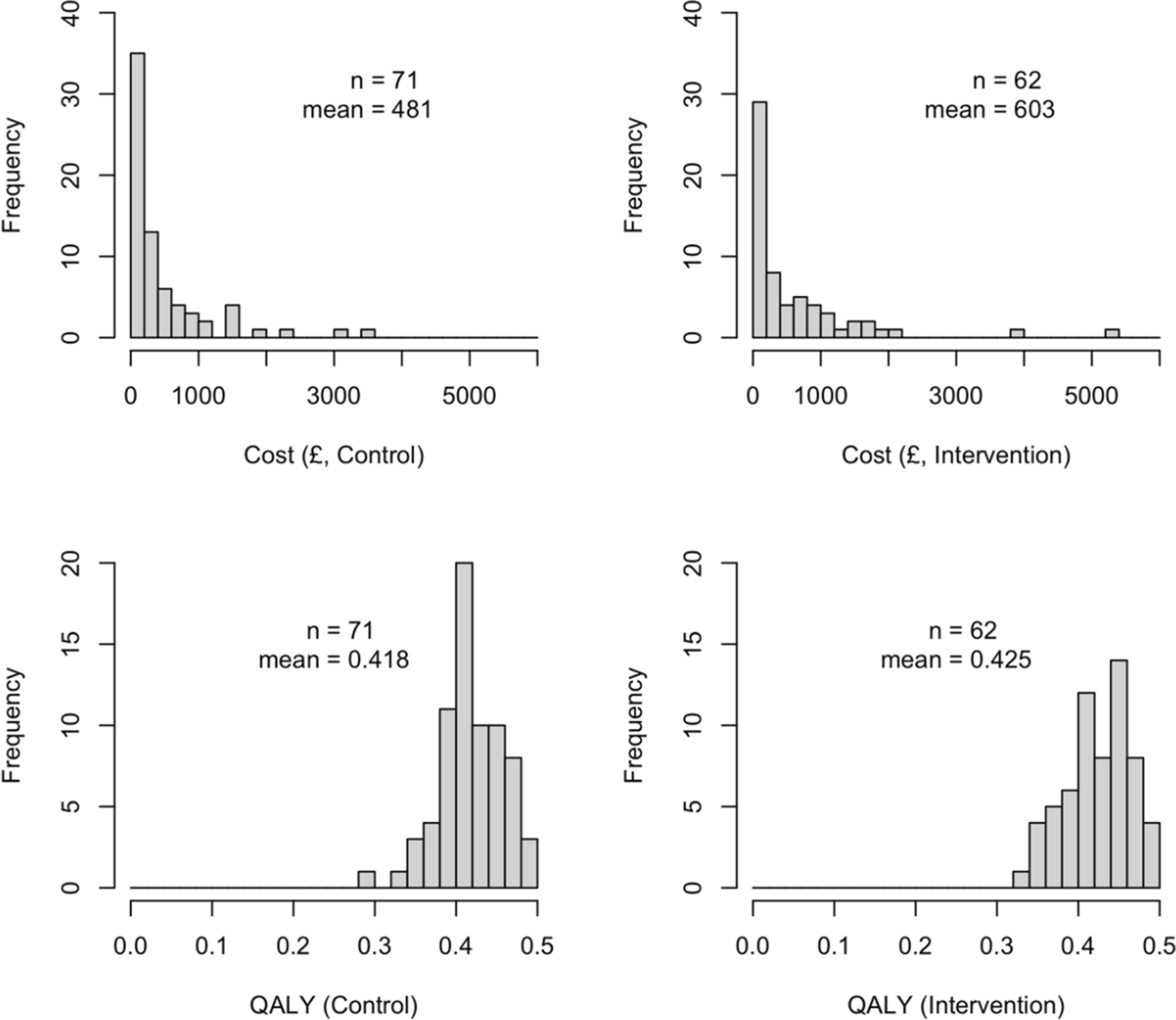
Complete cases, defined as patients with fully observed health care costs and utility scores at the three data collection time points, were used to streamline the analysis (71 in the control and 62 in the intervention). The decision was made because we concentrated on providing a comprehensive insight into how the choice of Uniform priors with various upper bounds can influence cost-effectiveness conclusions and considered that a complete case analysis was adequate to serve this purpose.

Analyses were performed within a Bayesian framework using a joint modelling approach [21]. The joint distribution of costs (\(c\)) and QALYs (\(e\)), denoted as \(p\left(c,e\right)\), was parameterised by the product of a conditional distribution of costs given QALYs, \(p\left(c\mid e\right)\), and a marginal distribution of QALYs, \(p\left(e\right)\), to capture the correlation between the outcomes. Apart from the Log-Normal distribution, Normal and Gamma distributions were considered for cost data to illustrate the extent to which different distributional assumptions can influence the impact of Uniform priors for cost standard deviations on cost-effectiveness results. Normal and Beta distributions were applied to QALYs; the former was chosen following the original health economic analysis of the trial, while the latter was used to reflect the potential skewness of QALYs.

The following notation was used: let \(_\) and \(_\) denote total costs and QALYs for patient \(i\) in each treatment arm \(t\) respectively. The treatment indicator \(t\) was dropped to simplify model specification.

The first model, assuming that both costs and QALYs are normally distributed, was undertaken to mimic the assumptions of routine CEAs. It can be thought of as a Bayesian equivalent to seemingly unrelated regression (SUR) [22] but re-expressed by using the aforementioned product formulation of the conditional distribution of costs given QALYs and the distribution of QALYs.

We modelled costs conditional on QALYs as:

$$\begin_\mid _ \sim }\left(_,_^\right)\\ _=_+_\left(_- }_\right)+_\left(_-\overline\right)+__\end$$

where \(_\) and \(_\) are the (individual-level) mean and the (population-level) standard deviation of the costs. Covariates were selected based on the original health economics analysis: \(\left( - \overline_ } \right)\) is the centred baseline costs, \(\left( - \overline} \right)\) is the centered QALYs while \(_\) is the site at which individual \(i\) has been treated. \(_\) is the intercept, \(_\) represents the impact of baseline costs on total costs, \(_\) quantifies the association between costs and QALYs while \(_\) represents the effects of site.

QALYs are modelled as:

$$\begin_ \sim }\left(_,_^\right)\\ _ =_+_\left(_- }_\right)+__\end$$

where the parameters \(_\) and \(_\) are the (individual-level) mean and the (population-level) standard deviation for QALY. In line with the original economic evaluation, centred version of utility values at baseline \(\left( - \overline_ } \right)\) and site \(_\) are included as covariates in the QALY model.

Suitable priors are specified for parameters to complete the model (see Appendix A for details and Appendix D for prior sensitivity assessment in the electronic supplementary material [ESM]); vague priors are assigned to the regression coefficients and Uniform priors are assumed for the standard deviations.

Since cost data are often right-skewed and non-negative, the cost component of the Normal model is expanded by assuming a Gamma distribution to reflect these features [23,24,25]. To facilitate prior specification and improve interpretability, the Gamma distribution for the costs given QALYs is re-parameterised by defining the shape parameter \(_=__\) and the rate parameter \(_=_/_^\), where \(_\) and \(_\) describe the (individual-level) mean and the (population-level) standard deviation of the costs, respectively. This parameterisation allows priors to be placed directly on more intuitive parameters such as cost standard deviation and avoids the difficulty of formalising straightforward prior knowledge for the shape and rate parameters. A log link function is used to connect the conditional mean costs given QALYs and relevant covariates. Since some participants accrued zero costs in the trial, we re-scale the observed values for the costs by adding a small constant \(\epsilon =1\) to the original data [8]. We note that modifying the data is necessary only to fit Gamma distributions to costs and has minimal impact on the conclusions under the overall scope of the study.

The costs conditional on the QALYs are modelled as:

$$\begin_\mid _ \sim }\left(__,_\right)\\ \text\left(_\right) =_+_\left(_- }_\right)+_\left(_-\overline\right)+__\end$$

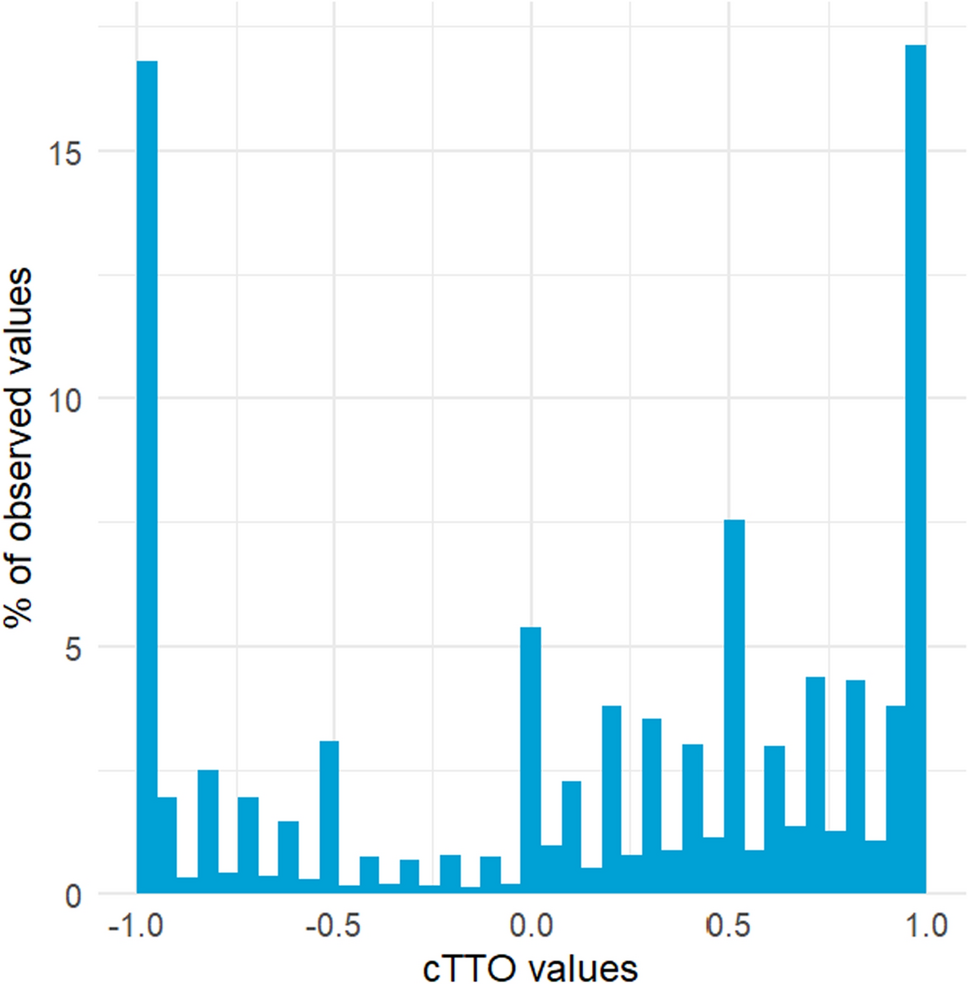
The QALYs’ empirical distributions also show some degree of skewness and are theoretically restricted within the range \(\left(0,0.5\right)\) in the ORBIT trial. Following the recommendation of previous research [26], a Beta distribution is fitted to the QALYs to capture the skewness of the outcome. The distribution of the QALYs is parameterised by two shape parameters, \(_=__\) and \(_=\left(1-_\right)_\), where \(_\) represents the (individual-level) mean while \(_\) is an (individual-level) scale parameter, defined as:

$$\begin_=\frac_\right)_}_^}-1\end$$

Such parameterisation allows construction of the priors directly on the standard deviations of the QALYs and brings more intuitive understanding of the model. A logit link function is applied for the generalised linear model.

The model for the QALYs can be expressed as:

$$\begin_ \sim }\left(__,\left(1-_\right)_\right)\\ }\left(_\right) =_+_\left(_- }_\right)+__\end$$

The model is completed by placing priors on the regression coefficients and the standard deviations: \(}\left(0,^\right)\) for the coefficients in the cost model, \(}\left(0,^\right)\) for the coefficients in the QALY model given the use of logit link; wide Uniform priors have been given to cost standard deviations—they have been selected to convey minimal information to the analysis and to ensure consistency with the Normal distribution choices for model comparisons throughout this study; although Uniform priors have been placed on the standard deviations of the QALYs, they are restricted using a \(}}\left(0,\sqrt_\left(1-_\right)}\right)\) due to the property of Beta distribution [4].

The model above is modified by assuming that the cost data are log-normally distributed, while maintaining the Beta distribution for the QALYs.

The cost Log-Normal model can be written as:

$$\begin_\mid _ \sim \text\left(_,_^\right)\\ _ =_+_\left(_- }_\right)+_\left(_-\overline\right)+__\end$$

It should be noted the \(_\) and \(_\) in the Log-Normal model are now (individual-level) mean and (population-level) standard deviation of costs on the log scale, respectively. To obtain the mean (\(_\)) and standard deviation (\(_\)) of costs on their original scale for each individual \(i\), the following expressions could be used:

$$\begin_ =\text\left(_+\frac_^}\right)\\ _ =\sqrt(_^)-1\right]\text\left(2_+_^\right)}\end$$

Similar to the Gamma distribution, the Log-Normal distribution requires the data to be positive, necessitating the addition of a small value (\(\epsilon =1\)) to the original cost data. Vague Normal prior distributions are assigned to regression coefficient parameters.

Uniform priors with different upper bounds are considered for the standard deviations of log costs in Log-Normal distribution (see Appendix A in the ESM) to assess their impact on the cost-effectiveness results. Specifically, to ensure the comparability across models with different distributional assumptions, the Uniform prior distributions on the log-cost standard deviation in the Log-Normal models are intended to lead to reasonable and comparable ranges to those on the original cost scale in other models. The exact upper bound values to be considered in the Log-Normal model may depend on the mean of the data, given the mathematical properties of the Log-Normal distribution. When the actual mean costs are large, a Uniform prior distribution with a large upper bound on log-cost standard deviation may produce unrealistic results. An illustration of the potential impact of the Uniform priors for log-scale standard deviation on original-scale standard deviation is provided in Appendix B (see ESM). Therefore, Uniform prior distributions with narrower and reasonable ranges have been chosen for the Log-Normal models, compared with those in the Normal and Gamma models.

All models are fitted in JAGS [27], a program for Bayesian inference based on Markov Chain Monte Carlo (MCMC) via the R2jags package in R version 4.0.3 [28]. We run two chains, each with 52,000 iterations, and discard the first 2000 iterations from each chain as a burn-in phase. A thinning rate of 10 has also been applied to reduce autocorrelation, leading to a total sample of 10,000 iterations for inference. Convergence is assessed through potential scale reduction statistics, \(\widehat\) [29], and a visual inspection on trace plots. To overcome the difficulty in model convergence arising from the differing scales of costs and QALYs, the original cost data have been scaled down by a factor of 10, but the resulting inferences are robust to the choice of the scaling factor. Model fit is assessed through posterior predictive checks (see Appendix C in the ESM) and compared by deviance information criterion (DIC) [30].

Given the main focus of our study, cost estimates are initially reported for the CEA models to identify how much the marginal mean costs can be affected by different upper bounds of the Uniform distributions. Mean costs with different distributional assumptions are also compared to investigate whether the influence brought by the Uniform prior distributions on cost standard deviations is sensitive to the choice of cost distributions. After that, the impact of using Uniform prior distributions on cost-effectiveness results is explored using a cost-effectiveness plane [31] and cost-effectiveness acceptability curve (CEAC) [32].