OmpK sequence

The OmpK protein of A. baumannii is a 241 amino acid protein for which there are several records on the NCBI server (https://www.ncbi.nlm.nih.gov/protein). In this study, the code CRL96222.1 of the A. baumannii OmpK sequence was used. By searching in the UniProt it was found that this protein is identical to TSX protein (Ion channel protein Tsx) with the code of A0A1S2FSG4_ACIBA.

Prediction and selection of epitopes

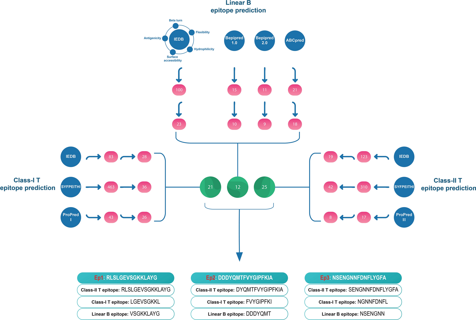
Since the use of multiple prediction tools increases the chance of obtaining more realistic epitopes, in this study several tools for epitope prediction were used. T-cell epitopes were predicted by three tools IEDB (http://tools.iedb.org), ProPred (http://crdd.osdd.net/raghava/propred/), and SYFPEITHI (http://www.syfpeithi.de/bin/MHCServer.dll/EpitopePrediction.htm). To predict these epitopes, the selection of HLA alleles with high frequency is needed, hence 10 class-I and 7 class-II HLA alleles with high frequency were used according to our previous experiences (Nemati Zargaran et al. 2021; Rostamian et al. 2020). These alleles were A*01:01, A*02:01, A*03:01, A*11:01, A*24:02, A*30:01, A*68:02, B*08:01, B*35:01, and B*51:01 of class-I and DRB1*03:01, DRB1*07:01, DRB1*15:01, DRB3*01:01, DRB3*02:02, DRB4*01:01, and DRB5*01:01 of class-II HLAs. All of these HLAs were among the 27 high-frequency alleles of the IEDB server (Greenbaum et al. 2011; Weiskopf et al. 2013), and according to the survey conducted on the allelefrequencies.net website (http://allelefrequencies.net/), they are among the high-frequency alleles in the whole world. The selected sequence length for predicting class-I and class-II T-cell epitopes was 9 and 15 amino acids, respectively.

Using selected HLA alleles and OmpK protein sequence as input in the epitope prediction portals of the prediction tools, several epitopes with different scores were identified. The threshold limit in IEDB was considered percentile rank ≤ 1 for class-I and ≤ 10 for class-II epitopes. For ProPred and SYFPEITHI, this threshold limit was considered to be a score above 10. A large number of predicted epitopes had to be filtered to reach a manageable number and the most likely ones were selected as epitopes. To perform this screening, first, the epitopes were clustered using the IEDB clustering tool (http://tools.iedb.org/cluster/) with a cut-off of 70%, and one epitope was selected from each cluster. This epitope had the highest prediction score or was predicted by more tools.

The prediction of linear B-cell epitopes was done as reported in detail in our previous work (Zargaran et al. 2020). In brief, using the seven epitope prediction tools in the IEDB website (http://tools.iedb.org/bcell/) as well as the ABCPred tool (https://webs.iiitd.edu.in/raghava/abcpred/), the primary possible epitopes were identified with scores from high to low. In the next step, epitopes with a high score in each tool were selected, and using the IEDB clustering tool, common epitope regions between the tools were identified and selected as possible linear B-cell epitopes.

After selecting the predicted class-I and II T-cell epitopes and linear B-cell epitopes, the sequences of all of them were aligned and clustered. The regions where all three types of epitopes (class-I and II T-cell and linear B-cell epitopes) were present were selected as the final epitopes of OmpK. These efforts led to the identification of three regions that contain potential T and B-cell epitopes and were named Ep1, Ep2, and Ep3. These three epitopes were used to design the multi-epitope vaccine constructs.

Characteristics of selected epitopes Ep1, Ep2, and Ep3

Cytokine response is mostly related to T helper cells that are stimulated by class II T-cell epitopes. Therefore, the possibility of producing three cytokines IFN-γ, IL-4, and IL-10 for class II T-cell epitopes present in selected epitopes Ep1, Ep2, and Ep3 was investigated. To predict IFN-γ production, the IFNepitope tool (https://webs.iiitd.edu.in/raghava/ifnepitope/application.php) was used. The IFNepitope tool predicts in three modes: 1- IFN-γ versus non- IFN-γ, 2- IFN-γ versus other cytokines, and 3- IFN-γ versus random. Each of these modes has different algorithms of SVM-based, Motif-based, or hybrid, which all of them were used in the present study.

The prediction of IL-10 and IL-4 cytokine responses was performed using the IL10pred server (https://webs.iiitd.edu.in/raghava/il10pred/index.html), and IL4pred server (https://webs.iiitd.edu.in/raghava/il4pred/predict.php), respectively. Various prediction algorithms provided by the servers were used. In no case, default parameters, including thresholds, were changed.

ToxinPred (https://webs.iiitd.edu.in/raghava/toxinpred/multi_submit.php) was used to predict whether the epitopes were toxic or not. The sequences of epitopes were placed as FASTA on the server portal. The server provides various prediction methods including SVM (Swiss-Prot) based, SVM (Swiss-Prot) + Motif based, SVM (TrEMBL) based, SVM (TrEMBL) + Motif based, Monopeptide (Swiss-Prot), Monopeptide (TrEMBL), Dipeptide (Swiss-Prot) and Dipeptide (TrEMBL). All of these methods were used and default parameters were not changed in any of them.

To check the allergenicity of Ep1, Ep2, and Ep3 epitopes, several tools including ALLerCatPro (https://allercatpro.bii.a-star.edu.sg/), SDAP (https://fermi.utmb.edu/), AllergenFP v1.0 (https://ddg-pharmfac.net/AllergenFP/), AlgPred (https://webs.iiitd.edu.in /raghava/algpred/submission.html), and AllerTOP v2.0 (https://www.ddg-pharmfac.net/AllerTOP/method.html) were used. In all the programs, the defaults of the tools were used.

Using the IgPred tool (https://webs.iiitd.edu.in/raghava/igpred/pep-fix-pred.html) it is possible to predict what type of antibody may be produced after encountering the epitopes. In the IgPred website, in the Epitope prediction section, the epitope sequences were entered as FASTA and the threshold limit remained at the same default (0.9 for all three types of IgG, IgA, and IgE antibodies).

Using the DeepTMHMM tool (https://dtu.biolib.com/DeepTMHMM) and without changing the defaults of the program, the topology and possible areas of transmembrane passage were predicted for the epitopes.

The PIR-International Protein Sequence Database (https://research.bioinformatics.udel.edu/peptidematch/batchpeptidematch.jsp) was used to check the cross-reactivity of epitopes Ep1, Ep2, and Ep3 with human proteome. In this server, Homo sapiens (9606) was selected as the type of organism, the sequence of epitopes was placed in FASTA format, and other parameters remained intact. Also, the degree of similarity of our epitopes with human proteome was checked by the BLASTP server (https://blast.ncbi.nlm.nih.gov/Blast.cgi?PAGE=Proteins). The two parameters Identity and Coverage were considered as criteria of similarity. If the epitope has a high percentage of similarity with the human proteome in both of these parameters, it should be removed.

HLA-epitope molecular docking

The binding of class-I and II T-cell epitopes present in Ep1, Ep2, and Ep3 (ligands) to their corresponding HLA alleles (receptors) was studied by molecular docking. For this purpose, the binding of allele HLA-A*02:01 (abbreviated A2, PDB ID: 5HHP) to class-I epitopes and allele HLA-DRB1*15:01 (abbreviated D15, PDB ID: 1BX2) to class-II epitopes were studied. Using PyMOL version 2.5.5, the receptors were prepared so that the chains bound to the ligand (chain A in the case of the A2 receptor and chains A and B in the case of the D15 receptor) were kept and the rest of the chains, water molecules, and any other additional molecules were deleted. Hydrogens were added to the remaining structures and saved in.pdb format for docking. The main ligands of 5HHP and 1BX2 files were used as docking controls.

The GalaxyPepDock server (https://galaxy.seoklab.org/cgi-bin/submit.cgi?type=PEPDOCK) was used for epitope-allele docking. The PDB file of the receptors and the FASTA format text file of the ligands were submitted to the server and it offers several complexes, the best of which was chosen as the most favorable docking complex. After docking and selection of complexes, they were refined with GalaxyRefineComplex server (https://galaxy.seoklab.org/cgi-bin/submit.cgi?type=COMPLEX) using default parameters. The server offers ten refined models for each complex, where model 1 had more favorable energy, hence selected as the final refined docking complex.

PRODIGY (https://wenmr.science.uu.nl/prodigy/) was used to analyze the results. This tool checks the binding affinity between the molecules of a complex. In this tool, the.pdb file of the complex was given, then the Interactor 1 part was selected as the primary chain involved in the binding, and for the Interactor 2 part, the second chain involved in the binding was added. The temperature was left at the server's default (25 °C) and then submitted. The results are presented in different formats including a table that contains useful information such as ΔG (kcal mol-1) and Kd (M) at °C. LIGPLOT + version 2.2.8 and PyMOL version 2.5.5 software were used to display the binding type as well as the residues involved in the binding.

Multi-epitope vaccine design

Using Ep1, Ep2, and Ep3 epitopes, several multi-epitope vaccine constructs were designed. For this purpose, β-defensin adjuvant and pan-HLA DR binding epitopes (PADRE) sequences were inserted to increase the constructs’ immunogenicity. EAAAK linker was used to connect adjuvant and PADRE sequences to each other and to other structures, and the GPGPG linker was used to connect epitopes. His-Tag sequence (6 histidine amino acid residues) was added to the constructs to purify the final protein by nickel column chromatography. Applying various epitope arrangements, four multi-epitopes were designed. Then these multi-epitopes were compared with each other and the best one was selected as the final vaccine construct. The positive selection criteria were better solubility, higher antigenicity, and more favorable molecular weight and physicochemical properties. Solubility was determined by Protein-Sol (https://protein-sol.manchester.ac.uk/), SolPro (http://scratch.proteomics.ics.uci.edu/Solpro), and PepCalc (https://pepcalc.com/). Antigenicity was predicted by the VaxiJen v2.0 (http://www.ddg-pharmfac.net/vaxijen/VaxiJen/VaxiJen.html). Molecular weight and physicochemical properties were estimated by the ProtParam tool (https://web.expasy.org/protparam/). The physicochemical properties predicted include isoelectric pH (pI), net charge, grand average of hydropathy (GRAVY), instability index, half-life, and Aliphatic index.

Investigation of multi-epitope properties

Some structural and physicochemical parameters of the final multi-epitope were estimated by inserting the sequence of the final multi-epitope as an input in the website http://scratch.proteomics.ics.uci.edu/. This website has collected several bioinformatics tools that predict different properties of proteins. Some of the tools of this website have been selected to predict the multi-epitope properties, including domains (with DOMpro tool), disordered regions (with DISpro tool), disulfide bonds (with DIpro tool), protein antigenicity (with ANTIGENpro tool), and solubility upon overexpression (with SOLpro tool).

The secondary structure of the multi-epitope was obtained from the PsiPred webpage (http://bioinf.cs.ucl.ac.uk/psipred/). In the same webpage, the DisoPred option was also checked so that disordered regions of the multi-epitope are predicted.

To predict toxicity, Toxinpred, to predict allergenicity, ALLerCatPro, SDAP, AllergenFP, AlgPred, and AllerTOP tools, to predict topology, DeepTMHMM, and to predict cross-reactivity with humans, PIR-International Protein Sequence Database were used. These tools were used as described above for single epitopes.

To more accurately predict multi-epitope localization, DeepLoc 2.0 (https://services.healthtech.dtu.dk/services/DeepLoc-2.0/), WoLF-PSORT (https://www.genscript.com/wolf- psort.html), and Hum-mPLoc 2.0 (http://www.csbio.sjtu.edu.cn/bioinf/hum-multi-2/) were used. In all cases, the defaults of the tools remained intact.

The full length original OmpK protein was used as control in all analyses.

Modeling and initial refinement of the multi-epitope

The Galaxy-TBM of the GalaxyWeb server (https://galaxy.seoklab.org/cgi-bin/submit.cgi?type=TBM) was used to predict and model the tertiary structure of the multi-epitope. In this server, the protein sequence was submitted and the server provided several models as more likely models of the protein's tertiary structure. The built models were saved in.pdb format and evaluated with SAVES v6.0 server (https://saves.mbi.ucla.edu/). In this server, there are several tools for evaluating the protein tertiary structure, including ERRAT, Verify3D, WhatCheck, and ProCheck. According to the evaluations of these tools, one of the constructed models received better scores, which was selected as the multi-epitope model and then subjected to initial refinement. Initial refinement of this model was done by GalaxyRefine (https://galaxy.seoklab.org/cgi-bin/submit.cgi?type=REFINE) and ModRefiner (https://zhanggroup.org/ModRefiner/). GalaxyRefine provided five models and ModRefiner provided one refined model, these models were also examined and compared by the SAVES server, and a model with better scores was selected as the initially-refined multi-epitope model.

Complementary refinement of the multi-epitope model by molecular dynamics simulation

To refine the model of the multi-epitope more accurately, the.pdb file of the initially-refined model was selected as input and subjected to complementary refinement using multiple tools.

These tools, all based on molecular dynamics (MD) simulations, include PREFMD (http://feig.bch.msu.edu/prefmd), locPREFMD (http://feig.bch.msu.edu/web/services/locprefmd/), FG-MD (http://zhanglab.ccmb.med.umich.edu/FG-MD/), and WebGro (https://simlab.uams.edu/). In all PREFMD, locPREFMD, and FG-MD tools, only the.pdb file of the protein was given to the server and the results were sent by email. In contrast, WebGro allows more choice. In this tool, which works based on MD simulation, refinement of the multi-epitope model was done twice, once using the GROMOS96 54a7 force field and once using the CHARMM 27 force field. Other parameters were selected as follows: Water model: simple point-charge (SPC), Box type: cubic, Salt type: NaCl (Neutralize and add 0.15M salt options were also checked), Integrator: Steepest descent, Steps: 5000, Equilibration type: NVT/NPT, Temperature: 300K, Pressure: 1 bar, MD integrator: Leap-frog, Simulation time: 50 ns (ns) and Approximate number of frames per simulation: 1000.

After the mentioned numerous refinements, the resulting models were compared by the SAVES server. Also, for a better comparison, PROSA-web (https://prosa.services.came.sbg.ac.at/prosa.php), QMEAN (https://swissmodel.expasy.org/qmean/), and Molprobity (http: //molprobity.biochem.duke.edu/index.php) were also used, in all of which the.pdb file was given as input.

On the QMEAN server, the QMEANDisCo option was selected which evaluates the local quality of the models and presents the results in the form of an overall score and several graphs. The Molprobity server provides several results, including the Ramachandran diagram and the overall Molprobity score, according to which a score below 1.5 means a structure with very good quality, between 1.5 and 2 is acceptable, and above 2 is weak (Chen et al. 2010). The PROSA-web server provides three graphs as a result: a z-score graph, a local quality model graph, and an interactive molecule viewer graph. In the z-score diagram, the models that have been identified based on x-ray and NMR have been brought and shown in light and dark blue colors on the diagram. The more the z-score is among the colored parts, the more similar it is to the real models, and in fact, the model is more accurate. In the diagram of the local quality model, the parts of the protein that give a positive number on the diagram mean that they are not of high quality, and the negative parts mean that they are more favorable in terms of energy. The interactive molecule viewer diagram depicts the three-dimensional structure of the protein and high-energy (red) and low-energy (blue) regions, where the blue regions are more favorable (Wiederstein and Sippl 2007).

By comparing the models refined by the quality assessment servers, one of the models that got more scores than the others, was selected as the final model of multi-epitope and used for further evaluations.

Multi-epitope conformational B epitope prediction

Conformational B epitope prediction was done with Discotop2.0 (http://tools.iedb.org/discotope/) and Ellipro (http://tools.iedb.org/ellipro/). The working principles were the same as in previous studies (Nemati Zargaran et al. 2021; Ranjbarian et al. 2023; Zargaran et al. 2020). In brief, the protein.pdb file was entered into each of the tools, and the results are presented in the form of graphs and tables. In the diagram, the places that are epitopes are in green above the threshold line and the places that are not epitopes are in red below the threshold line. The threshold was left as the tool's default. PyMOL software was used to demonstrate conformational epitopes using the information obtained from Discotop2.0 and Ellipro servers.

Codon optimization and multi-epitope in silico cloning

For codon optimization, the JCat server was used (http://www.jcat.de), in which the protein sequence was entered as an entry and E. coli (strain K12) was selected as the target organism. The results are presented as optimized codons and a graph. In the graph, there is a red line on the number 1, which is the most ideal codon state, if the codon is not optimal, it gives a negative peak towards the bottom of the diagram. In silico cloning of multi-epitope was done by SnapGene 3.2.1 software using the codon-optimized DNA sequence of the multi-epitope (insert) and the sequence of expression vector pET-21b ( +). The sequence of two enzymes, XhoI and NotI, was placed at two ends of the insert. Since the correct reading frame is messed up by adding the enzyme sequence, a random nucleotide (adenine) was added to the sequence. Also, for the correct termination of the translation, the termination codon (TAG) was placed at the end of the insert.

Immune response simulation

The C-IMMSIM server (https://kraken.iac.rm.cnr.it/C-IMMSIM/) simulated the immune response evoked by the multi-epitope. The FASTA format of the multi-epitope amino acid sequence was entered into the server and other parameters were selected as follows: the “Random seed part” left the same as the default, i.e. 12,345, the “Simulation Volume” part was the same as the default, i.e. 10, and the “Adjuvant” part was left as the default, i.e. 100. For “Simulation Steps”, 1050 steps were selected. In the “Host HLA selection” section, a mixture of high-frequency HLA alleles from class I and II (two from class I-A, two from class I-B, and two from class II-DR) should be selected. We, therefore, hit the following random but high-frequency alleles in order: A2:01, A11:01, B35:01, B51:01, DRB1:15, and DRB3:01. Three injections with an interval of four weeks were considered for simulation, and therefore, in the “Time step of injection” section, we added 1 time step for the first injection, 84 for the second injection, and 168 for the third injection (each time step is equal to 8 h). The vaccine without LPS was given in the “What to inject” section, The “Num Ag to inject” part, which is the injected antigen dose in microliters of the vaccine volume, was left as the default, i.e. 1000. Finally, the “submit job” button was pressed and the results, which were presented in the form of several charts, were saved. The full length original OmpK protein was used as control.

Molecular docking of multi-epitope-TLRs

The multi-epitope binding to toll-like receptor 2 (TLR2) and TLR4 receptors was performed by molecular docking study by HADDOCK 2.4 server (https://wenmr.science.uu.nl/). For this purpose, the structures of the ligand (the multi-epitope) and receptors (TLRs) were prepared and cleaned. The structure of the ligand was without extra chains and molecules, so only hydrogens were added to the structure. To prepare the receptors, the.pdb file for TLR2 (code: 2Z7X) and for TLR4 (code: 3FXI) was obtained from the RSCB PDB website (https://www.rcsb.org/). Then all molecules except for chain A (which represents the TLR molecule) were removed, hydrogens were added and the remained chains were saved as.pdb files.

To perform docking, we first obtained the active and passive residues involved in the interaction between the ligand and the receptor with the CPORT server available in HADDOCK (http://alcazar.science.uu.nl/services/CPORT/) using default parameters. CPORT uses five tools for predicting interaction regions, namely ProMate, PIER, SPPIDER, cons-PPISP, and PINUP, and presents the results as active and passive residues involved in binding (de Vries and Bonvin 2011).

Using the found active and passive residues and the prepared structures of receptors and ligands, molecular docking was performed with the HADDOCK 2.4 tool. For this purpose, protein–protein docking type was selected, and prepared.pdb files were used as input. The chains involved in binding and possible active and passive residues (as predicted by CPORT) were introduced to the server, and the rest of the default parameters of the server remained intact. The results were presented in the form of several clusters. Based on the sum of scores obtained from several parameters, it gives a general score called the HADDOCK score, the more negative the better, and sorts the clusters accordingly. The best cluster was selected as the final docking complex.

To refine the final docking complex, the HADDOCK website has a section called HADDOCK Refinement Interface (https://wenmr.science.uu.nl/haddock2.4/refinement/1) which water refined the complexes. The complex.pdb file was given and all other parameters were left intact as the tool defaults.

As mentioned for peptide-HLA docking, PRODIGY was used to analyze the docking results. The PDBsum server (http://www.ebi.ac.uk/thornton-srv/databases/pdbsum/) was used to display the atoms involved in the binding and the type of bonds. Beautification of docking complexes, interacting residues, and binding regions was done by PyMOL software.

Investigating the movement and deformability of multi-epitope-TLR complexes

Movement and deformability of docked multi-epitope-TLR complexes were performed by the iMODs tool (https://imods.iqfr.csic.es/). After obtaining the final multi-epitope docking complexes and TLRs, we gave the docked set to the server in.pdb format and the server makes the predictions. This server calculates several parameters such as deformability, B-factor, eigenvalues, and variance of multi-epitope-TLR complexes.