The Euclidean distance is a widely used metric and it is utilized mostly to examine the similarity degree between two objects that fall in the same class [42,43,44]. In mathematical terms it is expressed as the root of square difference between the co-ordinates of a pair of objects.

$$\:\begin_}_=\sqrt^_-_\right)}^}\end$$

(9)

Within the scope of this work, we utilized the SWAP quantum test [45] to compute the Euclidean distance between two state vectors A and B [46]. These two vectors reflect the ligand and the potential protein docking site states, accordingly, as explained in detail in the next section.

First of all, we have to properly encode our data into quantum states. Here, we utilized the quantum amplitude embedding technique to properly encode our data. We will elaborate more on this in Sect. 5.1 of this work.

$$\:\begin|A\rangle =\:\frac\sum\:__|i\rangle \end$$

(10)

$$\:\begin|B\rangle =\:\frac\sum\:__|i\rangle \end$$

(11)

Then we define states \(\:|\varPsi\:\rangle \) and \(\:|\varphi\:\rangle \) as follows:

$$\:\begin|\varPsi\:\rangle =\:\frac}\left[|0\rangle \otimes\:\:|\rangle +\:|1\rangle \otimes\:\:|\rangle \right]\end$$

(12)

$$\:\begin\:|\varphi\:\rangle =\:\frac}}\left[\left|\right||0\rangle -\left|\right||1\rangle \right]\end$$

(13)

Where \(\:Z=\:^+^\). Afterwards, we calculate the distance between states \(\:|\varPsi\:\rangle \) and \(\:|\varphi\:\rangle \) using the SWAP test operator. To do so, we have to apply the appropriate quantum circuit and then measure the qubit 0 state. The corresponding circuit will be discussed further in Sect. 5.4. Finally, the Euclidean distance between vectors A and B is computed as follows:

$$\:\beginD=\:\sqrt^}\end$$

(14)

The quantum algorithm

Our quantum algorithm consists of three main parts, namely the quantum search algorithm, the protein segmentation and shift and the identification and evaluation of docking sites part. The quantum search algorithm indicates whether there are any available potential docking sites, as well as their exact location, in side the given protein, as explained in detail in Sect. 3 of this work. The protein segmentation and shift part is used to examine all the possible docking sites within the protein. Finally, the evaluation of docking sites part, as the name implies, is used for the assessment of the potential docking sites regarding their similarity to the ligand. All the above can be summarized in the hierarchical flowchart of Fig. 5.

Fig. 5

Quantum algorithm hierarchical flowchart. A high-resolution image can be found in the supplementary material

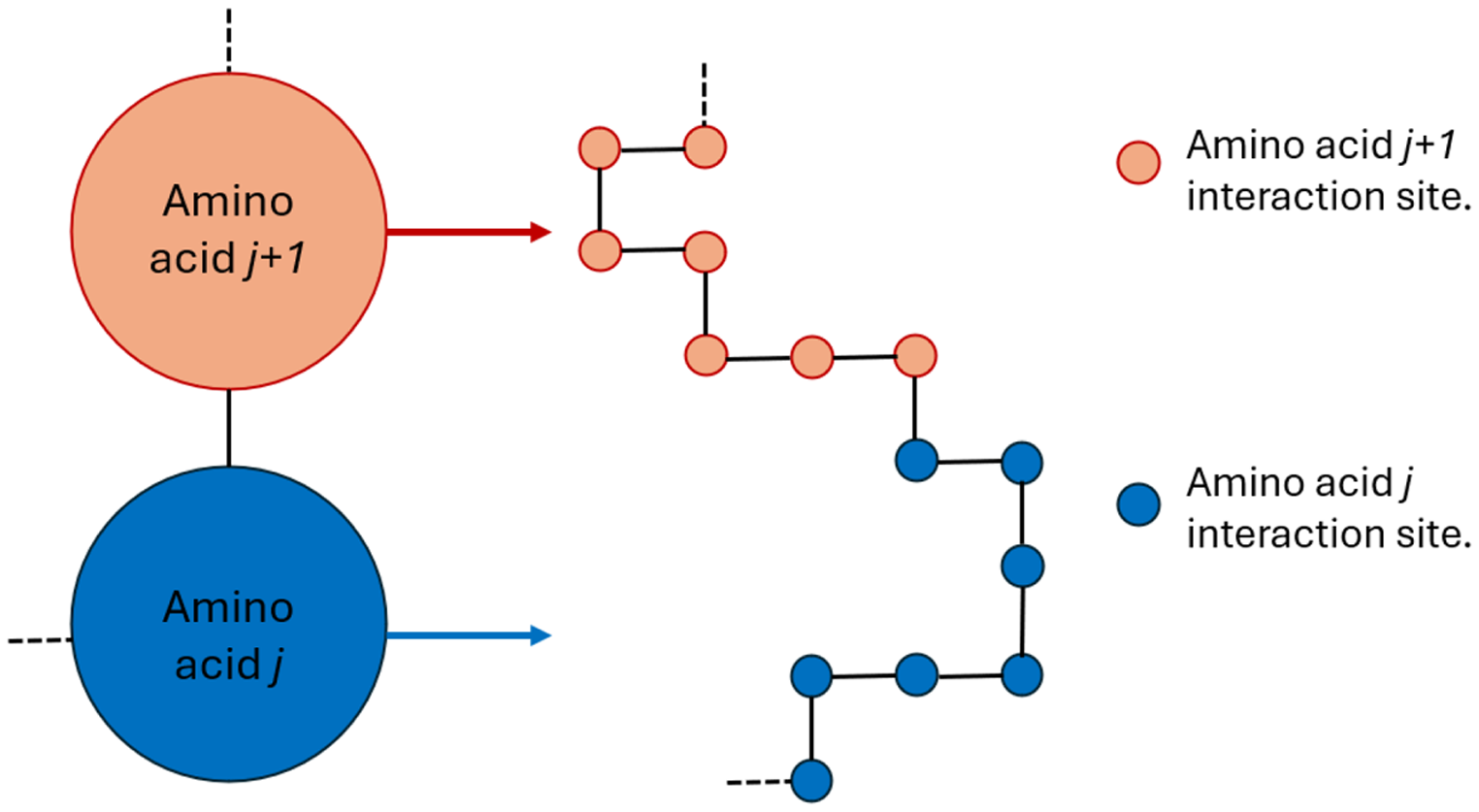
As mentioned in Sect. 2, we utilized two interactions of the ligand– protein interaction, i.e. “Hydrophobic interaction” and “Hydrogen bonding”, to describe each interaction site for both the ligand and the protein. These properties are described by continuous values which lie in a specific range bound by a minimum and a maximum value for each interaction. Thus, we considered two different encodings regarding the part of the problem they are referring to.

Hydrophobic interaction: \(\:[_,_]\)

Hydrogen bonding: \(\:[_,_]\)

First encoding

The first encoding is related to the quantum search algorithm. To describe an interaction site we utilized two qubits, each one corresponding to each of the two interactions, namely Hydrophobic interaction and Hydrogen-bonds. Thus, a quantum state of an interaction site is given by:

$$\:\begin|q\rangle =|_\rangle \otimes\:|_\rangle =|_q}_\rangle \end$$

(15)

where the left qubit corresponds to the hydrophobic interaction and the right one to the hydrogen bonding. The corresponding mapping of the properties’ continuous values to the quantum register is given by:

$$\:[_,\frac_+h}_})\:\grave\:\:|0\rangle $$

$$\:[\frac_+h}_},_]\:\grave\:\:|1\rangle $$

$$\:_,\frac_+hb}_})\:\grave\:\:|0\rangle \:$$

$$\:[\frac_+hb}_},_]\:\grave\:\:|1\rangle \:$$

An example of a ligand and a protein quantum state is presented below:

Ligand state example:

$$\:|_\rangle =|_\rangle \otimes\:|_\rangle \otimes\:|_\rangle =|11\rangle \otimes\:|01\rangle \otimes\:|10\rangle =|110110\rangle $$

Protein state example:

$$\eqalign\rangle &=|}\rangle \otimes|}\rangle \otimes|}\rangle \otimes|}\rangle \otimes|}\rangle \otimes|}\rangle \cr & =|11\rangle \otimes|11\rangle \otimes|10\rangle \otimes|01\rangle \otimes|10\rangle \otimes|10\rangle \cr & =|111110011010\rangle \cr} $$

Second encoding

The second encoding is related to the evaluation of the potential docking sites, identified by the quantum search algorithm. In the same manner, we utilize one qubit for each corresponding interaction, except now we consider it to be in quantum superposition of its basis states.

$$}\,}:[},}]\,\grave \,a|0\rangle + b|1\rangle $$

$$}\,}:[h},h}]\,\grave \,c|0\rangle + d|1\rangle $$

where a, b, c and d are the probability amplitudes and are given by:

$$\:\begina=\:\frac_-\:h}_\:-\:h\right|}^+_\right|}^}}\end$$

(16)

$$\:\beginb=\:\frac_}_\:-\:h\right|}^+_\right|}^}}\end$$

(17)

$$\:\beginc=\:\frac_-\:hb}_\:-\:hb\right|}^+_\right|}^}}\end$$

(18)

$$\:\begind=\:\frac_}_\:-\:hb\right|}^+_\right|}^}}\end$$

(19)

Thus, a quantum state for one interaction site is:

$$\:|q\rangle \:=|_\rangle =\left(\:a|0\rangle +\:b|1\rangle \right)\otimes\:\left(\:c|0\rangle +\:d|1\rangle \right)=$$

$$\:\begin=\:\:ac|00\rangle +\:ad|01\rangle +\:bc|10\rangle +\:bd|11\rangle \end$$

(20)

Protein segmentation and shift

To find the exact locations of the potential docking sites, we iteratively segment the protein described by the protein state into two parts as presented in Fig. 6. Again, we consider the size of the ligand to segment the protein.

Fig. 6

Protein segmentation according to the ligand size

For each segmented part of the protein, we utilize the protein superposition state that we have already described as an input to the modified Grover algorithm which we developed. The segmentation stops when the size of the ligand and the size, i.e. number of interaction sites, of the segmented protein parts are equal. At this point the algorithm deterministically indicates whether the corresponding interaction site is a potential docking site or not.

During the creation of the quantum superposition state, we considered the size of the ligand and created the corresponding basis states, taking into account the first interaction site as the starting point. In order to cover all the combinations of neighboring interaction sites, we utilized a shift component to our algorithm that creates a ‘new’ shifted protein, as shown in Fig. 7.

Fig. 7

For the newly created protein segmentation, the quantum search components will be applied, aiming to find additional potential docking sites. The shifting process is repeated iteratively until the ‘new’ created protein has not been a part of a previous search, or there are no more available interaction sites in the protein.

Identification and evaluation of potential Docking sites

After the potential docking sites have been identified, we evaluate them regarding their similarity to the ligand. As mentioned before, each potential docking site is of the same size as the ligand. Therefore, the second encoding for the state labels is utilized to create quantum state vectors for the ligand and the potential docking sites. These vectors are the quantum superposition of the ligand and potential docking sites’ basis states and probability amplitudes according to the real continuous values of the Hydrophobic interaction and Hydrogen bonding properties.

A straightforward approach to compare the similarity of these vectors is the Euclidian distance, as mentioned in Sect. 4. The ligand superposition state acts as the benchmark vector while the potential docking sites superposition states are those compared with the ligand. The site which is closer to the ligand superposition state returns the smaller Euclidian distance and it corresponds to the best available docking site.

For this reason, we considered the quantized version of the Euclidian distance computation as mentioned in the relevant section.

In respect of the initialization of the quantum register, we consider the amplitude encoding and thus, the \(\:|\varphi \:\rangle \) and \(\:|\psi\:\rangle \) states are given by:

$$\:\begin|\varphi\:\rangle =\frac}\left(\left|ligand\right|\left|0\rangle -\left|docking\_site\right|\right|1\rangle \right)\end$$

(21)

Where:

$$\:\beginZ=\:^+^\end$$

(22)

And

$$\:\begin|\psi\:\rangle =\:\frac}(|ligand\rangle \otimes\:|0\rangle \:+\:|docking\_site\rangle \otimes\:\left|1\rangle \right)\end$$

(23)

By performing the swap test and measuring the control qubit, we acquire:

$$\:_\left(0\right)=\:\left[|\varPsi\:\varphi\:\rangle +|\varphi\:\varPsi\:\rangle \right]\right|}^=\:\frac^=$$

$$\:\begin=\:\frac\left[\langle \varPsi\:\varphi\:|\varPsi\:\varphi\:\rangle +\langle \varPsi\:\varphi\:|\varphi\:\varPsi\:\rangle +\langle \varphi\:\varPsi\:|\varPsi\:\varphi\:\rangle +\langle \varphi\:\varPsi\:|\varphi\:\varPsi\:\rangle \right]\end$$

(24)

The following relation has been used:

$$\:\begin\langle \varPsi\:\varphi\:|\varphi\:\varPsi\:\rangle =\:\langle \varPsi\:|\varphi\:\rangle \otimes\:\langle \varphi\:|\varPsi\:\rangle =\langle \varphi\:|\varPsi\:\rangle \otimes\:\langle \varPsi\:|\varphi\:\rangle \end$$

(25)

Thus, based on Eq. 24, we derive the following:

$$\:\begin_\left(0\right)=\frac+\frac\langle \varPsi\:|\varphi\:\rangle +\langle \varphi\:|\varPsi\:\rangle =\frac+\frac^\end\:$$

(26)

By combining Eqs. 14 and 26, the Euclidian distance is given by:

$$\:\beginD=\:\sqrt_\left(0\right)-0.5\right)}\end\:$$

(27)

A technical detail that is worth to be mentioned is that the distance computation is based on the probability of finding the control qubit in state \(\:|0\rangle \). To improve the reliability of our results we opted for many shots on the quantum circuit execution and measurement. By doing this we reduced the statistical error percentage. The corresponding quantum circuit, as built in Qiskit, for the docking sites evaluation is shown in Fig. 8.

Fig. 8

Qiskit quantum circuit for the evaluation of docking sites

Implementation of the quantum algorithm

Our quantum algorithm has been implemented in IBM’s Qiskit framework (https://www.ibm.com/quantum/qiskit). Qiskit is a reliable and easy-to-use environment to develop and test quantum algorithms. Moreover, not only it provides a plethora of simulators where anyone can benchmark his quantum algorithms/circuits but also provides a convenient way to execute any quantum algorithm/circuit to IBM’s quantum computers [41].

Regarding the quantum search algorithm, i.e. the modified Grover search, for the protein superposition state as well as the quantum oracle, we utilized Qiskit’s built-in StatePreperation() and UnitaryGate() methods, respectively. Considering the Noisy Intermediate-Scale Quantum era (NISQ), we designed the Grover diffusion operator using two approaches. Both approaches yield the same results on Qiskit’s simulators.

In the first approach, we computed the Grover operator matrix, using Eq. 8, and utilized Qiskit’s built-in UnitaryGate() method to create the appropriate quantum gates, as shown in Fig. 9. The UnitaryGate() method transforms any unitary matrix to its corresponding quantum gates.

Fig. 9

Unitary matrix transformed to quantum gates

In the second approach, we opted for the amplitude amplification algorithm [47] to create the Grover diffusion operator as shown in Fig. 10. This approach requires an additional qubit for the quantum search circuit as presented in Fig. 11.

Fig. 10

The Grover diffusion operator

Fig. 11

The Amplitude amplification quantum circuit

Execution of the quantum algorithm on simulators

To test our algorithm’s capability to identify the location of the best docking site, we utilized the Sampler primitive that Qiskit provides. Moreover, we used appropriate values for the Hydrophobic interaction and Hydrogen bonding properties, for each one of the algorithm executions. All the following executions run on Qiskit’s simulators.

By utilizing the first quantum state encoding, the protein is shifted and segmented and the available docking sites are identified. While utilizing the second quantum state encoding, our algorithm identifies the best docking sites, as shown in Tables 1, 2 and 3.

Table 1 Algorithm execution results for a protein with 4 interaction sites and a ligand with 1 interaction siteTable 2 Algorithm execution results for a protein with 10 interaction sites and a ligand with 2 interaction sitesTable 3 Algorithm execution results for a protein with 27 interaction sites and a ligand with 3 interaction sites

It is worth mentioning that our algorithm is scalable and designed in such a way that its scaling corresponds to the ligand size and with the presented examples the scalability of the quantum algorithm is demonstrated. Larger proteins can be searched for as the number of available qubits increases.

Execution of the quantum algorithm on real IBM quantum computers

Apart from executing our quantum algorithm on Qiskit’s simulators, we also executed the algorithm on three real IBM quantum computers, all three comprising 127 qubits. More specifically, the quantum computers were the ‘ibm_brisbane’, ‘ibm_osaka’ and ‘ibm_kyoto’. We present the results of the first iteration, which involves searching the entire protein to identify the potential docking sites, for the ligand and protein given by:

$$\:|ligand\rangle =\:|1100\rangle $$

$$\:|protein\rangle =\:|010011001111000110100011\rangle $$

The expected probability of the state \(\:|1100\rangle \) according to the Qiskit simulation was 0.918. Yet, due to noise in the real quantum computer the probability distribution was affected by errors and led to a small improvement as shown in Fig. 12.

Fig. 12

Comparative results of the quantum algorithm execution for a protein with 12 interaction sites and a ligand with 2 interaction sites on real IBM quantum computer (‘ibm_brisbane’) and on the Simulator. Quantum hardware errors affect the probability distribution

We utilized two widely known quantum error mitigation techniques, namely the matrix-free measurement mitigation routine [48], known as M3, and the Pauli twirling technique [49], to improve the results. The former is a post-measurement technique for noisy input bitstring correction whereas the latter is a technique which reduces the coherent errors’ accumulation by converting arbitrary noise channels to Pauli channels during execution. Furthermore, to reduce coherent errors on idling qubits, during our quantum circuits’ execution, we applied the dynamical decoupling technique [50] with an XX pulse sequence. The hardware results show improvements, as shown in Fig. 13. Red color bars, denoted as ‘Raw’ in the legend, correspond to the original execution and all the others correspond to an error mitigated execution by applying a single or a combination of the techniques mentioned before. The best results were obtained by applying the dynamical decoupling technique during our algorithm execution.

Despite the hardware errors, the algorithm was executed correctly ensuring that the quantum algorithm will run without errors in the forthcoming fault-tolerant quantum computers.

Fig. 13

No-error (‘Raw’) and error mitigated results for the algorithm execution on ‘ibm_brisbane’. As depicted, either a single or a combination of the techniques mentioned were applied. The ‘DD-XX’ abbreviation stands for Dynamical Decoupling with XX pulse sequence. This technique yielded the best results overall, by eliminating a portion of the existing noise